I strongly recommend reading the previous blog post before diving deep into this one.
When it comes to HTTP clients in Elixir the first option would be HTTPoison. HTTPoison
is a wrapper around Erlang HTTP client called hackney. According to the hex.pm, HTTPoison
is the most popular HTTP client in Elixir. In fact, before Mint release, HTTPoison
was the only Elixir/Erlang HTTP client which does proper SSL verification by default, out of the box. HTTPoison
provides a simple and straightforward interface to send HTTP requests, hiding all the complexity of establishing a connection, maintaining a connection pool and so on.
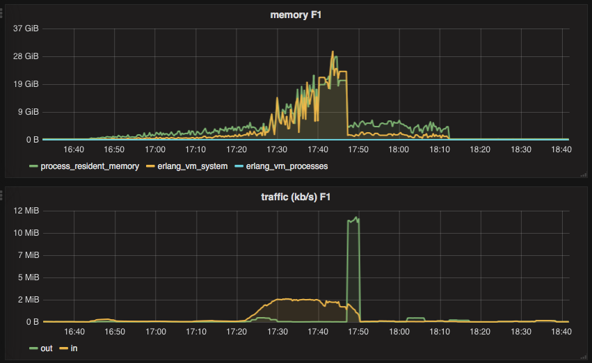
However, we’ve encountered some issues with hackney
. Occasionally hackney
could get stuck, so all the calls to HTTPoison
would be hanging and blocking caller processes. It would look like on the graph below.
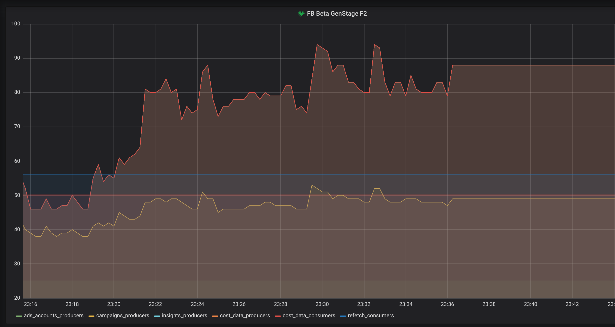
As you can see the new GenStage processes are not spawned anymore because all of the already spawned processes are blocked by the calls to HTTPoison
. The only way to get out of this state was to restart hackney
app using Application.stop/1
and Application.start/1
functions. Most likely the problems we’ve encountered are related to this issue.
Thankfully by the time we started looking around for an alternative HTTP client, Gun reached 1.0.0 version. Gun
is an Erlang HTTP library from the author of Cowboy. Gun
provides low-level abstractions to work with the HTTP protocol. Every connection is a Gun
process supervised by Gun
’s Supervisor (gun_sup
). A request is simply a message to a Gun
process. A response is streamed back as messages to the process which initiated a connection. Full documentation could be found here. The asynchronous nature of Gun
allows performing HTTP requests with multiple connections without locking a calling process. Gun
does not provide a connection pool, so you should manage connections manually.
Here is how we implemented Gun
based HttpClient
module in our app.
1 2 3 4 5 6 7 8 9 10 11 12 13 14 15 16 17 18 19 |
|
:gun.open/3
creates a new connection (a new gun
process) to the given host
and port
. Once the process is started and a connection is established, gun
process sends back a gun_up
message which is caught by :gun.await_up/2
. At this point, gun
process is ready to receive requests.
We call HttpClient.connection/2
function upon CampaignProducer
start because CampaignProducer
is the first process in the GenStage pipeline which actually sends an HTTP request.
1 2 3 4 5 6 7 8 9 10 11 12 13 14 15 16 17 18 19 20 21 22 23 24 25 26 |
|
This way CampaignsProducer
is an owner of Gun
process, so all it will receive are messages from Gun
. Once CampaignProducer
gets all the campaigns from Facebook, it passes them down the pipeline and spawns more GenStage workers which also send requests to Facebook. The idea here is that all the children GenStage processes would send subsequent requests to Facebook using this one connection created by CampaignProducer
process. Thus the number of CampaignProducer
across all Facebook accounts equals to the number of Gun
workers/connections and it means we can control it. Let me show it on a scheme from the previous blog post.
+----------+ +----------+ +----------+ |Insights | |CostData | |CostData | +---> |Producer <----+Producer <----+Consumer | | | | |Consumer | | | | +----------+ +----------+ +----------+ | +------------+ +-----------+ +----------+ +----------+ +----------+ |Campaigns | |Campaigns | |Insights | |CostData | |CostData | --|Producer <-----+Consumer +--> |Producer <----+Producer <----+Consumer | | | |Supervisor | | | |Consumer | | | +------------+ +-----------+ +----------+ +----------+ +----------+ | | +----------+ +----------+ +----------+ | |Insights | |CostData | |CostData | +---> |Producer <----+Producer <----+Consumer | | | |Consumer | | | +----------+ +----------+ +----------+
CampaignProducer
initiates a new Gun
connection, sends a request to Facebook to get campaigns and passes them down the pipeline. InsightsProducer
and CostDataProducerConsumer
use Gun
’s connection they received from CampaignProducer
and pass it to HttpClient
’s get/2
and post/3
functions in order to send HTTP requests. It’s worth noting that sending a GET or POST request in this case does not spawn any new processes or connections. All the GenStage workers spawned by CampaignProducer
send HTTP requests by utilizing the same Gun
connection. When all campaigns are consumed, CampaignProducer
closes Gun
connection and dies with the normal
state. Effectively, we’ve built a pool of Gun’s connections within the existing GenStage pipeline!
Let’s see how sending GET and POST requests with Gun
would look like.
1 2 3 4 5 6 7 8 9 10 11 12 13 14 15 16 17 18 19 20 21 22 23 24 25 26 27 28 29 30 31 32 33 34 35 36 37 38 39 40 41 42 43 44 45 46 47 48 49 50 51 52 53 54 55 56 57 58 59 60 61 62 63 64 65 66 67 |
|
That’s quite a lot of code. Gun
’s documentation highlights it as well stating the advantages a developer has with such an architecture.
While it may seem verbose, using messages like this has the advantage of never locking your process, allowing you to easily debug your code. It also allows you to start more than one connection and concurrently perform queries on all of them at the same time.
Sending a request is basically sending a message to a Gun
worker (conn_pid
variable in our example). Then the process which initiated a connection starts to receive a response as messages from Gun
process. A request is uniquely identified by stream_ref
, so it’s important to pattern match against it in receive do
block. Receiving the full response is achieved by receiving messages from Gun
process till the :fin
mark.
Please note, that the implementation above does block the process while the process is waiting for a message inside receive
block. Having receive
block was suffice for our case. In order to avoid any process locking, you should implement receive
block via GenServer’s handle_info
callbacks.
As I mentioned above, HTTPoison
is the only Elixir/Erlang library which does a proper SSL certificates verification by default. In order to instruct Gun
to do so as well, you need to provide certain options to :gun.open/3
function.
1 2 3 4 5 6 7 8 9 10 11 |
|
:certifi and :ssl_verify_hostname dependencies should be listed in your mix.exs
.
Gun
is a low-level HTTP client which is quite verbose and looks a bit awkward at first glance. However, it provides low-level abstractions to work with HTTP, giving you full control over connections and allowing you to receive responses asynchronously without locking your processes. And this is exactly what you need when you send millions of HTTP requests per day. The most important thing in our case was the ability to control connections and split them between different branches of GenStage pipeline. This way any single dropped connection does not impact others making our app resilent to HTTP errors.
Recently two Elixir Core contributors @whatyouhide and @ericmj announced the first stable release of Mint, the very first native Elixir HTTP client. This is a big deal to Elixir community if you ask me. Mint
does SSL verification by default and shares the same principles as Gun
. However, while Mint
has the same basic idea as Gun
, the fundamental difference is that Mint
is completely processless. Gun
has Supervisor gun_sup
which spawns Gun
’s workers which hold connections. Every connection is a Gun
process. Mint
does not have that, a connection in Mint
is just a struct. I’m looking forward to trying Mint
in one of our projects in the future.
In today’s blog post I would like to show how using a proper back-pressure mechanism helps us send millions of HTTP requests to Facebook per day and how we implemented it using GenStage.
One Adjust account can have multiple Facebook accounts associated with it. A client adds Facebook accounts using OAuth authentication through Adjust MMP (Mobile Measurement Partner) Facebook app. Every Facebook account can have multiple so-called AdsAccounts. Clients use individual AdsAccounts to run their Facebook campaigns. The information about campaigns performance is available via Facebook Ads Insights Marketing API. Having Facebook accounts integrated with proper credentials and AdsAccounts synced, one can finally fetch data from Facebook. We picked Elixir as the implementation language for the project responsible for getting data from Facebook.
The original implementation used the easiest and the most straightforward way to run code concurrently in Elixir - Task.async
. We would iterate through all Adjust accounts which have Facebook accounts and spawn one process per Adjust account. Then in each of these processes, we would fetch data from Facebook concurrently firing HTTP requests to Facebook for all Facebook AdsAccounts available. One request — one task. Then all tasks are sent to Task.await
, the fetched data is put into a queue and a Processor
process is started per every Adjust account_id
. Each Processor
process gets the data from the queue, does some additional transformations and stores the data to the database.
As you can see, the original implementation was pretty straightforward: get all AdsAccounts, fetch the data using Tasks.async
/Task.await
, put the fetched data into the queue and process it.
However, over time, we started to observe the limitations of this architecture. We got more and more clients with Facebook accounts integrated, meaning we would spawn more and more concurrent processes to fetch Facebook data. Not only Facebook API was not happy about getting so many of these requests but our service also was struggling to digest all these processes and data fetched.
Whenever you need a back-pressure mechanism in Elixir, the answer is obvious, it’s GenStage
. I like the wording from the GenStage announcement:
In the short-term, we expect GenStage to replace the use cases for GenEvent as well as providing a composable abstraction for consuming data from third-party systems.
This is exactly what we needed: fetching a lot of data from 3rd party service with back-pressure in place.
GenStage
brings a concept of Producer and Consumer. A Producer has events in its state and Consumer subscribes to the Producer and consumes events according to some rules. GenStage
comes with a variety of different behaviours for Consumers which dictate the way how events are going to be consumed. Once Consumer is subscribed to Producer, it demands events from Consumer and Producer handles the demand in handle_demand/2
callback. However, handle_demand/2
is not the only place from where Producer can send events to Consumer. handle_call/3
, handle_info/2
and handle_cast/2
callbacks have an additional element in the return tuple, so they can send events to Consumer too! Another important detail to note is that once Consumer asked for demand from Producer, it never asks for more demand till it gets all the events it asked previously.
GenStage
can provide us with back-pressure, but how does it fit with the task at hand? To illustrate that let me introduce steps involved in the processing.
As you can see, there a lot of repetition of ‘for each’ statement meaning every one ‘event’ from the previous step produces more ‘events’ down the stream. Another important detail to note is that Facebook API has the quota per Facebook account and per Facebook AdsAccount, meaning after eating 100% of the quota Facebook API starts sending errors instead of actual data in the response.
For our purpose, ConsumerSupervisor behaviour seemed to be the perfect fit. It works like a pool, but every consumed event has its own separate process. ConsumerSupervisor would restart crashed processes and would demand more events once min_demand
processes terminate with :normal
or :shutdown
status. We could adapt it to our needs, this is how the very beginning of our flow looks like.
+------------+ |AdsAccounts | +--->+Producer | | | | | +------------+ | +----------+ +-----------+ +------------+ | Accounts | |Accounts | |AdsAccounts | | Producer +<-----+Consumer +--->+Producer | | | |Supervisor | | | +----------+ +-----------+ +------------+ | | +------------+ | |AdsAccounts | +--->+Producer | | | +------------+
AccountsProducer
is a part of the application’s Supervisor tree, so it’s started when the app is started. It fetches active Facebook accounts from the database and puts them into its state. AccountsConsumerSupervisor
is also a part of the application’s Supervisor tree and it is subscribed to the AccountsProducer. Once AccountsProducer
gets the Facebook accounts in its state, AccountsConsumerSupervisor
starts to consume them and spawn a process per each Facebook account consumed. From the code perspective, it looks like the following.
1 2 3 4 5 6 7 8 9 10 11 12 13 14 15 16 17 18 19 20 21 22 23 24 25 26 27 28 29 30 31 32 33 34 35 36 37 38 39 40 41 42 43 44 45 46 47 48 49 50 51 52 53 54 55 56 57 |
|
1 2 3 4 5 6 7 8 9 10 11 12 13 14 15 |
|
The initial number of events to demand and the number of events to trigger for more demand are specified by max_demand
and min_demand
options respectively. This allows us to control how many Facebook accounts we would like to process at once. Each AdsAccountProducer
gets an event (Facebook account_id) from AccountsProducer
. Once started, AdsAccountsProducer
fetches from the database all Facebook Ads accounts which belong to given Facebook account and then puts them into its state. AdsAccountsProducer
uses Registry to name processes. Using Registry
allows us to comply with Name registration restrictions. Also, we poll Registry
to report a number of alive workers to the metrics collection system.
1 2 3 4 5 6 7 8 9 10 11 12 13 14 15 16 17 18 19 20 21 22 23 24 25 26 27 28 29 30 31 32 33 34 35 36 37 38 39 40 41 42 43 44 45 46 47 |
|
Great, now we can ‘produce’ and ‘consume’ Facebook accounts, but what’s next? Each AdsAccountsProducer
holds some AdsAccounts in its state, but there are no consumers which would consume them to continue the flow. So why not to spawn consumers dynamically per AdsAccountProducer
and use the same ConsumerSupervisor
logic further?
+------------+ |Campaigns | +---> |Producer | | | | | +------------+ | +------------+ +-----------+ +------------+ |AdsAccounts | |AdsAccounts| |Campaigns | +---> |Producer | <----+Consumer +--> |Producer | | | | |Supervisor | | | | +------------+ +-----------+ +------------+ | | +-----------+ +-----------+ +------------+ | +------------+ | Accounts | |Accounts | |AdsAccounts | | |Campaigns | | Producer | <-----+Consumer +--> |Producer | +---> |Producer | | | |Supervisor | | | | | +-----------+ +-----------+ +------------+ +------------+ | | +------------+ | |AdsAccounts | +---> |Producer | | | +------------+
Starting consumer dynamically would require adding AdsAccountsConsumerSupervisor.start_link(account_id, self())
to handle_info/2
in AdsAccountsProducer
, so it would start a consumer for itself after it puts AdsAccounts into its state. The self()
among the arguments is required so AdsAccountsConsumerSupervisor
knows a process it needs to subscribe to.
1 2 3 4 5 6 7 8 9 10 11 12 13 14 15 16 17 18 19 20 |
|
Every AdsAccountProducer
starts its own consumer, which would consume AdsAccounts and spawn CampaignProducer
per each Facebook AdsAccount. CampaignsProducer
gets AdsAccount and a date to fetch, then it asks Facebook API for active campaigns which are running under given AdsAccount for given date. And then finally it puts campaigns into its state and, you guessed it, starts a consumer for itself.
+------------+ |Insights | +---> |Producer | | | | | +------------+ | +------------+ +-----------+ +------------+ |Campaigns | |Campaigns | |Insights | +---> |Producer <-----+Consumer +--> |Producer | | | | |Supervisor | | | | +------------+ +-----------+ +------------+ | | +------------+ +-----------+ +------------+ | +------------+ |AdsAccounts | |AdsAccounts| |Campaigns | | |Insights | +---> |Producer <-----+Consumer +--> |Producer | +---> |Producer | | | | |Supervisor | | | | | | +------------+ +-----------+ +------------+ +------------+ | | +-----------+ +-----------+ +------------+ | +------------+ | Accounts | |Accounts | |AdsAccounts | | |Campaigns | | Producer | <-----+Consumer +---> |Producer | +---> |Producer | | | |Supervisor | | | | | +-----------+ +-----------+ +------------+ +------------+ | | +------------+ | |AdsAccounts | +---> |Producer | | | +------------+
Every InsightProducer
gets a Facebook campaign_id
, fetches Insights from Facebook Marketing API and puts the fetched data into its state.
Unfortunately, InsightsProducer
cannot store data yet. A Facebook campaign’s insights represents data per day, whereas at Adjust we have to store this data per hour because of timezones support. Therefore a Consumer for InsightsProducer
needs to issue an additional HTTP request to Facebook API for every Ad to get hourly distribution. The fact that we have quite a lot of Ads to ask hourly distribution for imposes some limitations to the way how we can consume Insights from every InsightsProducer
. Consuming the events from InsightsProducer
the same way using ConsumerSupervisor behaviour would generate a lot of concurrent requests to Facebook even if max_demand
would be 2, so quota would be consumed quite fast. Therefore the Consumer for InsightsProducer
should consume events slowly and check quota after every request. Fortunately, GenStage comes with manual
mode, which allows consuming events explicitly. Once a Consumer is set into manual
mode, there is no max_demand
and min_demand
anymore, one should ask for events explicitly instead.
+----------+ +----------+ +----------+ |Insights | |CostData | |CostData | +---> |Producer <----+Producer <----+Consumer | | | | |Consumer | | | | +----------+ +----------+ +----------+ | +------------+ +-----------+ +----------+ +----------+ +----------+ |Campaigns | |Campaigns | |Insights | |CostData | |CostData | +---> |Producer <-----+Consumer +--> |Producer <----+Producer <----+Consumer | | | | |Supervisor | | | |Consumer | | | | +------------+ +-----------+ +----------+ +----------+ +----------+ | | +------------+ +-----------+ +------------+ | +----------+ +----------+ +----------+ |AdsAccounts | |AdsAccounts| |Campaigns | | |Insights | |CostData | |CostData | +---> |Producer <-----+Consumer +---> |Producer | +---> |Producer <----+Producer <----+Consumer | | | | |Supervisor | | | | | |Consumer | | | | +------------+ +-----------+ +------------+ +----------+ +----------+ +----------+ | | +-----------+ +-----------+ +------------+ | +------------+ | Accounts | |Accounts | |AdsAccounts | | |Campaigns | | Producer | <-----+Consumer +---> |Producer | +---> |Producer | | | |Supervisor | | | | | +-----------+ +-----------+ +------------+ +------------+ | | +------------+ | |AdsAccounts | +---> |Producer | | | +------------+
CostDataProducerConsumer
is set to manual mode, it’s started by InsightsProducer
, demands one event (one ad), sends a request to Facebook API, gets the data and passes it to the CostDataConsumer
which finally stores it to the database. After every request to the Facebook API, CostDataProducerConsumer
checks quota values in the response headers: if the quota is nearly depleted, it demands a new event from InsightsProducer
with some delay using Process.send_after/3
. Otherwise, if the quota values allow, it does that immediately. Also, a Consumer of InsightsProducer is actually a ProducerConsumer, because it both consumes and produces events. Here is how one can set a Consumer or ProducerConsumer into the manual
mode.
1 2 3 4 5 6 7 8 9 10 11 12 13 14 15 16 17 18 19 20 21 22 23 24 25 26 27 28 29 30 31 32 33 34 35 36 37 38 39 40 41 42 43 44 45 46 47 48 49 50 51 52 53 54 55 56 57 58 59 60 61 62 63 64 65 66 67 68 |
|
That is finally the end of the flow. So far it looks like the following:
AccountsProducer
is started by the main Supervisor, gets accounts from db, puts into its stateAccountsConsumerSupervisor
is started by the main Supervisor, it subscribes to AccountsProducer
, consumes events (accounts) and spawn one AdsAccountProducer
per each accountAdsAccountsProducer
fetches Facebook account’s AdsAccounts from the database, puts them into state and starts dynamically a ConsumerSupervisor for itselfAdsAccountsConsumerSupervisor
consumes AdsAccounts, spawns one CampaignsProducer
per each AdsAccountCampaignsProducer
gets AdsAccount, fetches active campaigns from Facebook API, puts them into its state and starts a CampaignsConsumerSupervisor
for itselfCampaignsConsumerSupervisor
consumes campaigns, spawns one InsightsProducer
per each campaignInsightsProducer
gets campaign’s Insights from Facebook API, puts the data into its state and starts a consumer for itselfInsightsProducer
is CostDataProducerConsumer
, it’s set into manual
mode and consumes events one by one, for every consumed event (an ad) it sends additional HTTP request to Facebook API, gets the data and passes it further to CostDataConsumer
CostDataConsumer
gets all the data, does some transformations (timezone conversion, currency conversion, etc) and puts data into the databasePhew. That’s a lot happening here, but although it might look complicated, in fact, the architecture is quite simple. The same ConsumerSupervisor behaviour was applied several times to run multiple Facebook Accounts, AdsAccounts and Campaigns processes concurrently and without blocking each other.
Now, the question is how and when a producer process exits with :normal
or :shutdown
status, so ConsumerSupervisors can demand more events and spawn more processes. So let’s follow the termination path, i.e. how these GenStage processes get terminated. Let’s start with the last part: InsightsProducer
- CostDataProducerConsumer
- CostDataConsumer
. CostDataProducerConsumer
demands events from InsightsProducer
one by one and passes the events down the flow to the CostDataConsumer.
Every time an event is consumed, CostDataProducerConsumer
asks its InsightsProducer
how many events are left in its state. When the answer is zero, CostDataProducerConsumer
sends an event to CostDataConsumer
indicating that there was the last event. Let’s see how it would be implemented in handle_events/3
callback from the listing above.
1 2 3 4 5 6 7 8 9 10 11 12 13 14 15 16 17 18 19 20 21 22 23 24 25 26 27 28 |
|
After that CostDataConsumer
has 10 seconds to finish processing and storing the last batch of the events. After 10 seconds it terminates itself with :normal
status.
1 2 3 4 5 6 7 8 9 10 11 12 13 14 15 16 17 18 19 20 21 22 23 24 25 26 27 28 29 30 31 32 33 34 35 36 37 38 39 40 41 |
|
Since CostDataConsumer
, CostDataProducerConsumer
and InsightsProducer
are linked using start_link/3
, termination of CostDataConsumer
would terminate InsightsProducer
and CostDataProducerConsumer
with the same status. Once InsighsProducer
goes down with :normal
state, CampaignsConsumerSupervisor
can demand more campaigns from CampaignsProducer
and spawn more InsightsProducers
for the new campaigns.
Now let’s see how CampaignsProducer
and AdsAccountsProducer
terminate itself. The logic is the same for both of these producers, so let me show in detail how CampaignsProducer
exits with :normal
state. CampaignsProducer
checks its state every 5 seconds and when there are no more campaigns in its state to process and there are no InsightsProducers
active, it exits with :normal
state, which allows AdsAccountsConsumerSupervisor
to spawn more CampaignsProducer
for the newly consumed AdsAccounts.
1 2 3 4 5 6 7 8 9 10 11 12 13 14 15 16 17 18 19 20 21 22 23 24 25 26 27 28 29 30 31 32 33 34 35 36 37 38 39 40 41 42 43 44 45 46 47 48 49 50 51 52 53 54 55 |
|
AdsAccountsProducer
has the same logic, the only difference is ConsumerSupervisor name in consumers_alive?/2
function.
The only GenStage processes which never goes down (unless there is an exception) are AccountsProducer
and AccountsConsumerSupervisor
. Once the number of accounts in AccountsProducer
is closing to zero, it repopulates its state with more accounts from the database, so it never stops producing events.
GenStage
allows a developer to build sophisticated data flows with back-pressure in place. It provides necessary abstractions for producing and consuming events. In combination with Registry
, we could build a robust application which can fetch and process Facebook cost data for thousands of different AdsAccount without blocking each other. Every AdsAccount, Campaigns or Ad is processed separately from each other and if any of processes crashes, GenStage’s ConsumerSupervisor would restart it. The application can dynamically speed up or slow down the flow by itself based on Facebook quota values.
This blog post got long enough already and I even haven’t started to talk about one of the most important part of the application — HTTP client. We send over 6 millions of heavy, long-lasting HTTP requests to Facebook per day, so having a reliable and fast HTTP client is vital. This is going to be a topic for my next blog post. Stay tuned!
]]>We found unexpected and severe whole system pauses during the garbage collector’s mark phase. This was an surprising, as Go widely advertises itself as having a low pause garbage collector. In particular we found that the expected ‘stop the world’ pause was very short, but that whole system pauses experienced during the mark phase were several orders of magnitude longer. Observing that these pauses exist is important for understanding why we see such a large performance impact from GC cycles when there are plenty of CPU resources available and the reported pauses are very short.
In this post we will detail what we saw during this experiment and discuss how this impacts the way we investigate GC performance for all of our systems going forward.
It is worth noting that the system measured here was compiled with Go version 1.10. As the GC algorithm is under constant development these effects may disappear in later releases.
In order to compare the behaviour of this application (we will call it the MT command) we will be using the go trace
tool. We will narrow our definition of system performance to the rate of ‘network events’. This is an attractive metric because it appears directly in the trace itself and because the MT command’s main behaviour is making requests to two datastores, so any disruption to the performance of the MT command should be reflected here.
Each trace is taken while forcing a GC cycle. This guarantees that we can trace the behaviour we are interested in.
Because the trace tool is primarily visual we will only perform a visual analysis. There are no statistics used to interpret any of these results. Being able to inspect the trace tool output numerically would be a valuable development.
We will look at the traces with three different heap sizes. The heap size is described by a range as the heap size is constantly fluctuating due to memory being allocated and GC cycles completed.
We will look at 3 different states of our running program, During GC, Stop The World Pause and Behaviour After GC. The system behaviour during GC is the most interesting, here we see unexpected, and unexpectedly long, whole system pauses.
During GC the rate of network events (indicated by the red arrow) becomes very choppy, with frequent large blank gaps. Below the Network/Syscalls rows we saw three ‘Dedicated GC’ threads and a number of other threads which are a mix of Idle GC
(dull red) and useful work (green and blue). Although not pictured here the remaining threads were dominated with Idle GC
slices (here the word ‘slice’ refers to the period a goroutine was scheduled in a trace) with useful work being spread out across all threads.
With a medium sized heap we saw a very similar trace during GC. Again we saw that the rate of network events is very choppy, with frequent large blank gaps.
The largest heap size shows the same characteristic gaps as the previous smaller heaps.
When we looked closely at the mark phase pauses we found that at each heap size they were of roughly similar size. Here we show one in detail. The ~19 millisecond pause (indicated by the red arrow) shown here shows how large these gaps can be. It should be noted that this gap was chosen because it was particularly large and probably indicates a rough worst case pause. But other gaps were much larger than 1 millisecond and very frequent.
The final ‘stop the world’ pause is very short. Of a different order of magnitude compared to the pauses experienced during the mark phase above.
Another very short stop the world pause.
Here again the stop the world pause is very short. The pauses at the end of the mark phase was very short. As widely reported.
Here we compare the system performance outside of GC cycles at different heap sizes. We see no clear difference at different heap sizes, which is pretty much what you would expect.
At the smallest heap size we saw a solid block of network events over a 100 millisecond period. Without GC running we get very constant performance with no large breaks in network events. Below the Network/Syscalls rows we saw the MT command running comfortably with many short running goroutine slices (top level green/blue slices) paired with syscalls (red slices just below).
With a medium sized heap we saw the same behaviour.
With a 60-70 GB heap the GC cycle ran for almost 10 seconds and our trace only ran for 5 seconds so we didn’t capture any ‘after gc’ trace. We do have a GC-less trace when the heap ranged 95-105 GB. We will use that to observe the ‘normal’ behaviour with a very large heap.
Even at this very large heap size we see the same normal system performance.
Here we zoom into a typical millisecond to get a feel for the normal rate of network events. Although we only present a sample from the 95-105 GB heap, the ‘normal’ rate of network events was very similar at all heap sizes we tested. It is interesting to relate this typical 1 millisecond period back to the large (up to ~20 millisecond) gaps we saw during GC. For every millisecond of pause we experience we are missing out on a very large number of network events.
We have seen the impact of a GC cycle in the trace taken directly from the running MT command. But does it have any observable impact outside the command itself? If the impact was only visible in a detailed trace then we would not need to worry about these different behaviours. We can look at the metrics reported by one of the datastores to observe the increasing impact on performance as the heap grows.
With a 8-15 GB heap we saw small shallow drops in read/write rates.
With a 98-107 GB heap we saw larger and deeper drops in read/write rates from the datastore’s perspective.
Go’s GC algorithm is advertised widely as having very low pauses. When people talk about GC pauses in Go applications they typically talk only about the ‘stop the world’ pause which occurs at the end of the mark phase. Our tests agree that this pause is very short, but we also experience clear and repeated pauses which are much larger than this during the mark phase. These pauses are much more interesting to us when trying to diagnose performance issues which may be GC related. Unfortunately these mark phase pauses are totally unreported by any of the standard metrics reported by the Go runtime and garbage collector.
The size of the mark pauses appear to be roughly similar at different heap sizes. The biggest impact heap sizes have is on the duration of the GC cycle itself. At 8-13 GB GC took 1.5 seconds to complete, at 20-30 GB GC took 4 seconds and at 60-70 GB heap GC took 12 seconds. This means that we experienced performance disruptions for longer periods the more the heap grew. It is particularly interesting to see a very large number of ‘Idle GC’ slices in each trace. The test was performed on a single machine with 48 cores. Execution without GC required roughly 2-4 cores, but with GOMAXPROCS unset the MT command could use all 48 cores. During GC it appears to try to use all available CPU cores, but most of them remain idle. The issue we see here could be the scheduler struggling to effectively schedule a very large number of non-performing GC goroutines.
If we want to understand the performance of Go systems with large heaps we cannot rely on the standard set of metrics. At this time we don’t know of any way to observe these performance degradations except by manually viewing traces, which is very awkward and time consuming. Further developments here would be very beneficial.
]]>This blog post is the first in a series on this extension. In it I cover the difficulties which come with creating tooling around utility statements in PostgreSQL as a whole, why centralising this in user defined functions is a good idea, and what kinds of problems we are trying to solve.
In the next article in this series, we will cover the major implementation details. In that post, we will discuss how we prevent SQL injection from occurring within user-defined functions, both in terms of language injection and object injection. We will also areas of development in this area which have, for now, not been included in the extension and the security problems they pose. In the final article in the series, we will discuss the unique testing needs of such a security critical piece of infrastructure, the tooling available, and the difficulties we ran into in trying to ensure that the tests run consistently on various versions of PostgreSQL.
This blog post includes sample ways of doing things which are wrong but are included in order to communicate problems that happen. Please resist the urge to copy and paste, and instead make sure you understand what you are doing. Things like placeholders may be handled in different ways depending on different database drivers, for example.
PostgreSQL has supported the standard database role-based permissions model since PostgreSQL 8.1. In this model we think about granting access to roles, and also granting one role to another. Depending on how roles are defined, they may pass on permissions to child roles automatically or not. Managing the permissions given to various roles is an important part of securing a PostgreSQL database.
All permissions are managed by a part of the SQL language known as DDL or “Data Definition Language.” A typical set of role management statements might look like:
1 2 3 4 5 6 |
|
Now, on the surface these look like they pose no problems for automated tooling, but how do we ensure that a schema, table, or role name is handled in a correct way and is not a vector for SQL injection or other bad things?
A naive approach might be to try to use placeholders where you want to supply input but this doesn’t work for a couple of reasons. The first is that placeholders are intended for literal values only and typically we want to interpolate identifiers and SQL key words.
If the database driver sends the data separately from the query then the parse tree will be invalid. If the client interpolates client-side, the escaping will be incorrect because of the complexities in rules for escaping portions of the query. SQL identifiers have an escaping syntax that is related to but different from the escaping of string literals, and you cannot escape keywords.
1 2 3 4 5 |
|
But, you may say, there is one case where you have a string literal (the password). Unfortunately that does not always work but for a different reason: in PostgreSQL, to have a parameterised query you have to put it through the whole planning pipeline. Utility statements, unfortunately have no plan attached.
1
|
|
Now if this is interpolated on the client, then things are handled properly, but if interpreted on the server, you will get a syntax error.
Now, trying to parameterise these things is something that comes up periodically, in various forums. People often do want to create roles from the application. Sometimes this is because of a desire to create database roles for application uses to let the database enforce security, and sometimes (as here) it is to try to improve tooling for setting up the database users across a series of servers.
The only way you can run DDL statements in PostgreSQL is via string concatenation. This opens up the issue of SQL injection in the tooling used to create and manage roles. This is particularly true if you have an automatic job that looks for new tables and ensures ownership is correct. For example if a malicious user created a table or function with a problematic name, it might be possible to inject sql into the script. For example:
1 2 3 |
|
In a case like this, a naive script might run and try to assign ownership to Postgres by using simple string interpolation:
1 2 3 |
|
If I then drop the table after becoming superuser, maybe nobody ever notices…
The same trick can be done even if naive escaping of the identifier is done. In other words, it is no different, really, than any other sort of SQL injection except that most of the tools we have to combat the problem are not of any use.
PostgreSQL provides functions for escaping identifiers, but these cannot be safely used inside client-side string interpolation without extra round-trips to the server and they don’t apply to SQL keywords.
The goal, simply, is to be able to use our ordinary SQL injection toolkits for role management, and to ensure that the complexity of the queries we are issuing for role creation are kept to an absolute minimum.
In other words, instead of our previous example, it would be better to do this:
1 2 3 4 5 6 |
|
Suddenly all the queries are parameterised, and we can use all our normal anti-sql-injection tools. Additionally, rather than dealing with a different syntax for each type of statement, we have a consistent semantic structure, making tool creation much easier.
Finally in doing this we can place the responsibility for safe operation to the functions we call and only require that we pass in something valid. This helps guard against changes in our tools introducing accidental vulnerabilities.
On the server-side, PostgreSQL provides a very rich set of tools for preventing SQL injection. These include parameterised queries where possible (including with dynamic SQL in PL/PGSQL), solid escaping functions for both literals and identifiers, and some handy data-types which eliminate SQL injection in some cases. By using these methods effectively as applicable, we can reduce our original problem to one which is widely supported (where we pass in string literals into parameterised queries, even for role management functions).
As we have already noted, parameterised queries, server-side don’t apply to many of our cases, but there are two cases where they are very Helpful, namely in error handling and passing control between functions in the extension.
More frequently we will use escaping functions like quote_literal()
and quote_ident()
as well as types which represent strings bound to
catalog entries, such as regclass
and regprocedure
. These types
not only ensure proper escaping, but when strings are passed into the
user-defined functions, they also ensure that the corresponding
database object exists and is found (numbers cast to OID’s however
are not so checked).
None of these tools address keywords, however. For keywords, we use a whitelist system. This means we have to add new keywords to the white lists as they are supported by PostgreSQL but it also means we are protected against SQL injection issues through this vector.
In addition to our immediate use case, there were a few other use cases I knew of that I worked on supporting to ensure that the extension could be of use beyond Adjust. These all fit in with the idea that roleman should be safe toolkit for managing roles, and that it should do this job well.
Among others, supported use cases include:
Create simple scripts for creating SQL commands for role management to be run via psql. This requires restricting identifiers to the subset that does not require escaping.
Safely manage roles via application code. Applications that want to delegate security to the database have a safe framework for doing this.
A safe framework for database users to alter their own passwords with appropriate administrator-supplied security policies. Note that we are not doing this at Adjust but I know of others who are.
In the first case, you have the added complication that you cannot rely on the server-side protections against SQL injection to prevent SQL injection (though you can rely on client-side escaping of string literals). This is not our responsibility and roleman already makes the situation better by opening up more tools to be used to assure secure operation in this case.
The third case offers a particular problem, that any function which calls
roleman.set_password()
must do so in a security definer context. This means
further that we must test against database object injection, not merely
SQL language injection. In general the security guarantees that supporting
scenario require are worth the extra effort in supporting them. Besides,
someone will probably use the module in this way at some point so it is better
if they don’t run into trouble over it.
SQL object injection is a form of SQL injection that we will discuss in more detail in the next post, as well as how to prevent it. As of Roleman 0.2.1 we specifically test against a wide range of SQL injection techniques including injecting objects that shadow expected objects. Version 0.2.1 is believed to be safe when properly used.
I hope you have enjoyed this article.
Next we will discuss the implementation of this extension. We will also discuss the various techniques used to tighten and ensure security against a wide range of attacks.
]]>null
when we didn’t expect it or a good old side effect in a presumably clean function. Tests are considered first-class citizens in our code base and are mandatory for any pull request that adds or changes functionality.
Just like tests, any dependency that we bring into our projects becomes a part of our code base. Since no one likes maintaining code written by some unknown dude (do you?), we try to reduce the number of third-party packages we use to an absolute minimum and prefer writing or own tailor-made libraries.
This is why we decided to stick with the minimalistic but decent testing
package that Go provides as a part of its standard library.
Every test, regardless of programming language, contains four major parts: setup, invocation, assertion, and teardown. Besides providing the framework to run tests using the go
tool, testing
provides only one of these things–assertion–and leaves the rest up to its user. While the invocation part is usually very specific to implementation and there is not much that could be generalized there, setup and teardown are tightly coupled and can often be split into small reusable blocks that mock external services, provide data fixtures, etc. So we’ll focus on these two parts, specifically on mocking HTTP requests to external services.
A common task in our tests is to verify the interaction with an HTTP API provided by a third party. We don’t want to send all the requests we’re making in our unit tests to an actual server for several reasons:
Thus we came up with a fairly simple idea to mock http.Client
:
1 2 3 4 5 6 7 8 9 10 11 12 |
|
Now we only needed to mock the expected requests with canned responses:
1 2 3 4 5 6 7 8 9 10 11 12 13 14 15 16 17 18 |
|
1 2 3 4 5 6 7 8 9 10 11 |
|
This approach worked well for a while, but soon we found ourselves adding more and more functionality to testutils.ClientMock
. Sometimes we’d need to add additional cookies to the response, send requests using different HTTP methods, or provide a different response depending on what was sent in the request. The mock became so complex, that we started thinking about writing tests for it.
Nobody was smitten with the idea of writing tests for tests, so we had to rethink our approach. By that time, our client mock looked almost like a limited http.Server
without the transport part, so we decided to leave the honorable task of testing mocks to the Go team and came up with the following approach, which is currently used in most of our tests these days:
1 2 3 4 5 6 7 8 9 10 |
|
And the code turned into something like this:
1 2 3 4 5 6 7 8 9 10 11 12 13 14 15 16 17 18 19 20 21 22 |
|
We’re now using the standard library *http.Client
, and, instead of mocking its request methods, we override the host and port of the API server. This way we can redirect every HTTP request to our server mock:
1 2 3 4 5 6 7 8 9 10 11 12 13 14 15 16 17 18 19 20 |
|
For tests that explicitly require HTTPS, we added a similar mock that creates an instance of httptest.Server
by calling httptest.StartTLSServer()
instead of httptest.StartServer()
, while the rest of the code is completely the same as in testutil.ServerMock()
:
1 2 3 4 5 |
|
But this made http.Client
complain about a bad certificate:
1 2 |
|
Since we did not provide any certificates at all while creating an httptest.Server
instance, there should have been some default one hidden in net/http/httptest
. It turned out that the Go standard library contains a self-signed certificate and a private key used by the httptest
package. So we needed to make the http.Client
trust this certificate:
1 2 3 4 5 6 7 8 9 10 11 |
|
If you’ve already upgraded to Go 1.9, then you don’t need x509.ParseCertificate()
anymore. An instance of httptest.Server
now has a Certificate()
method that returns an *x509.Certificate
used by this server.
All that was left now was to replace the system-default http.Client
certificate pool with our own one, which held our server mock certificate:
1 2 3 4 5 6 7 8 9 10 11 12 13 14 15 16 17 18 19 20 21 22 23 24 25 |
|
Since Go v1.6, http.Server
supports HTTP/2 out of the box, and we naturally assumed httptest.Server
would, too. However, once we configured http.Client
to use http2.Transport
from golang.org/x/net/http2
, our tests that used testutil.ServerMock()
began to fail with an unexpected error:
1 2 3 |
|
A quick note on ALPN ALPN or Application-Layer Protocol Negotiation is a TLS extension that allows parties to agree on which protocol should be handled over a secure connection. HTTP/2 uses this feature to avoid additional round trips, and, hence, TLS handshakes, by agreeing on an application protocol during the hello phase. The client provides a list of protocols it supports and the server is expected to choose one and send it back.
So unexpected ALPN protocol ""; want "h2"
meant that our server did not know it now supported HTTP/2. There is a method in the http2
library to configure an existing server to support HTTP/2, but it expects an instance of http.Server
as an argument, whereas we only had httptest.Server
. Passing (httptest.Server).Config
as an argument to http2.ConfigureServer()
wouldn’t work, because httptest.Server
uses Config
to serve incoming connections using an already existing tls.Listener
that is created when (*httptest.Server).StartTLS()
gets called, and ALPN support is implemented by crypto/tls
. Thus we needed a way to configure the httptest.Server
listener to support "h2"
as an application-level protocol.
1 2 3 4 5 6 7 8 |
|
Looks exactly like what we’re looking for! What was left was to apply the same configuration changes as http2.ConfigureServer()
does and we’d have a nicely working HTTP/2 mock using Go standard library only:
1 2 3 4 5 6 7 8 9 10 11 12 13 14 15 16 17 |
|
Here, http2.NextProtoTLS
is a constant for the "h2"
string we were looking for and tls.TLS_ECDHE_RSA_WITH_AES_128_GCM_SHA256
is a cipher suite required by the HTTP/2 specification.
Instead of mocking http.Client
, mock the server it talks to. The Go standard library offers a very convenient net/http/httptest
package that allows you to spawn an HTTP server with only a few lines of code, which can be easily configured to handle HTTP/2 requests.
json
or csv
blobs and sometimes they are as big as a few hundred megabytes. Because of this, downloading such a report via API gateway just to send it to a client does not sound like a good idea. Below, you can see what happened to our naïve implementation when a number of clients were trying to download sizeable reports.
In this blogpost, I’d like to describe how we’ve implemented transparent streaming of HTTP requests directly to a client.
In the above screenshot, the “Traffic” graph perfectly illustrates what happens without streaming: an application receives data from a requested service for quite a while (yellow line, “in”), and once all the data is there, it sends it to a client (“out” line). With the streaming approach, there should be no significant gaps between the “in” and “out” lines on this graph, because the API gateway should send a chunk to the client as soon as that chunk is received from the requested service.
Due to past decisions at Adjust, our application already had HTTPoison in its dependencies list, which meant we already had hackney installed in our app, so we decided to try and implement HTTP streaming based on it. hackney
provides an async
option to receive a response asynchronously, but more importantly it allows us to pass {:async, :once}
so we can process the next chunk of a response only when the previous chunk has been processed. HTTP streaming with hackney
can be achieved using the following snippet:
1 2 3 4 5 6 7 8 9 10 11 12 13 14 15 16 17 18 19 20 21 22 23 24 25 26 27 28 29 30 31 32 33 34 35 36 37 38 39 40 41 |
|
Once a request to a service is sent, hackney
starts to send messages to a calling process. After receiving an initial response from the service, the API gateway calls the Plug.Conn.send_chunked/2
function, which sets proper headers and the state to conn
. Then, every time the calling process receives a new response chunk, it sends this chunk to a client using Plug.Conn.chunk/2
. If the chunk/2
function returns {:error, :closed}
, the client most probably just closed a browser tab. send_error/2
here is the custom function, which sends an error to error tracking service.
That code did what we’d hoped and worked well for us in most cases. But soon we noticed that sometimes this code behaved as though it wasn’t streaming data, but instead first accumulated the entire response and then sent it to a client. When this happened, hackney
consumed a lot of RAM, making an Erlang node unresponsive.
We spent quite some time investigating the issue and figured out that this behaviour was somehow related to cached responses. The whole investigation and its results deserve a separate blog post. In fact, @sumerman is preparing one with all the details about nginx
caching, hackney
streaming implementation details and more. Stay tuned!
In the meantime, we decided to replace hackney
with ibrowse
to see if it made any difference. And it did.
For ibrowse there is HTTPotion — a simple Elixir wrapper. We switched all our simple requests without streaming to HTTPotion
and implemented streaming with ibrowse
for reports, as in the code snippet below.
1 2 3 4 5 6 7 8 9 10 11 12 13 14 15 16 17 18 19 20 21 22 23 24 25 26 27 28 29 30 31 32 33 34 35 36 37 38 39 40 41 42 43 44 45 46 47 48 49 50 51 52 53 |
|
As you can see, the snippet for ibrowse
looks very similar to the one for hackney
. ibrowse
gives you a stream_to
option as well as the once
parameter, which allows you to control when to get the next response chunk. Unfortunately, HTTPotion
does not support the stream_to: [{pid, :once}]
option directly. Instead, you have to pass it via the ibrowse
option, but then all the messages coming from the ibrowse
process are not converted to the corresponding HTTPotion
structures. That’s why you have to pattern match against raw ibrowse
messages.
We found that streaming with ibrowse
worked very well. In cases when hackney
started to consume a lot of RAM, ibrowse
managed to keep memory consumption under control. Even when the gateway streams ~26 megabytes per second, memory usage stays stable around ~250 MB.
Look at the “Traffic” graph: the “in” and “out” lines are so close you can’t even see the green “out” line. Perfect!
Moreover, ibrowse
gives you more control on how you want to process and stream chunks. For example there is stream_chunk_size
parameter that lets you set your desired chunk size. There is also a spawn_worker_process/1
function, so it’s possible to create a separate worker for streaming per domain. You can find all the possible options in the ibrowse
wiki.
HTTP streaming using ibrowse
worked so well for us, that we haven’t even had a chance to try gun. According to its documentation, gun
has been designed with streaming in mind, so you might like to give it a try.
That’s it for today, folks. Happy streaming!
]]>http
library with fasthttp
. Fasthttp is a low allocation, high performance HTTP library, in synthetic benchmarks the client shows a 10x performance improvement and in real systems the server has been reported to provide a 3x speedup. The service we wanted to improve makes a very large number of HTTP requests and so we were very interested in using the fasthttp
client.
In the course of making the switch we encountered a number of difficulties. First the fasthttp
library presents a very different interface to the programmer which must be adjusted to. Second there were a number of quirks in the implementation which made progress rather slow.
To begin with we would like to learn how to perform a simple HTTP request using the fasthttp
client. Below is a very simple request using the Go standard library, error handling has been omitted for brevity.
For all the code snippets below the test server writes the request’s “User-Agent” header value and body into the response on separate lines. We write the actual output of the snippet in comments beneath each print statement.
1 2 3 4 5 6 7 8 9 10 11 |
|
A fasthttp
request can be written, also without error handling, very similarly:
1 2 3 4 5 6 7 8 9 10 11 12 13 |
|
The body of an http.Response
is exposed as an exported io.ReadCloser
field. The body of a fasthttp.Response
is exposed via the Body()
method call which returns a []byte
. The implication of this is that the entire body must be read and a sufficiently large []byte
allocated before the body can be processed. This is a surprising feature of a library which prioritises performance and low memory allocations.
One curious aspect of the Body()
method is that it returns no error, in contrast to reading from an io.ReadCloser
. It would be interesting to see how that method is implemented to get a better idea of how fasthttp
works.
1 2 3 4 5 6 7 8 9 10 11 12 13 14 15 16 17 18 19 20 21 22 23 24 25 26 27 28 29 30 31 32 33 34 |
|
The Body()
method operates on two unexported fields body
and bodyStream
. It first checks if bodyStream
is non-nil, and if it is, reads from the bodyStream
into the body
field. Finally the contents of the body
field are returned to the caller.
This is pleasantly straightforward, but there is one odd wrinkle, this method will silently eat errors.
Looking at line 15 in the example above we can see that any errors encountered while reading from bodyStream
are written into the body
field and the original error is not returned. An error could occur, but we would never find out about it. Lets look further into our simple HTTP request example to see how the Body()
method would actually execute.
If we trace the execution of our simple request above we find the following execution path:
1 2 3 4 5 |
|
Inside ReadLimitBody(...)
we find this critical piece of code
1 2 3 4 5 6 7 |
|
We can see, on line 3, that the call to readBody(...)
sets the bytes bodyBuf.B
to be the result of reading from the connection. So the stream reader field will be nil. We can see that errors are being returned from the readBody(...)
method call. That’s good, but we have only covered one simple case. From further analysis I do believe that errors are not swallowed by the fasthttp
client, but I am not certain. There is a potential execution path which results in errors being silently swallowed.
Our existing application performs both GET and POST requests. We ran into a small problem making POST requests. We will start with a simple POST example using fasthttp
. Here we set our method to POST and fill in the body with some form-encoded values. Now we see both the “User-Agent” and the non-empty request body in the response.
1 2 3 4 5 6 7 8 9 10 11 12 13 14 15 |
|
Next we want to set our “User-Agent” header manually, but there is a small problem.
1 2 3 4 5 6 7 8 9 10 11 12 13 14 15 16 |
|
While the standard library http.Client
does provide a default “User-Agent” header value, this value is overridden when any other value is provided. Fasthttp is still sending it’s default “fasthttp” and our “Test-Agent” value is not being picked up.
We wanted to get a better look at the headers that were being set, so we added a single debug line println(req.Header.String())
. Now we can no longer ignore errors in our code, because that innocent looking req.Header.String()
causes client.Do(...)
to fail.
1 2 3 4 5 6 7 8 9 10 11 12 13 14 15 16 17 18 19 20 21 22 23 |
|
When we print the request headers we get to see the preloaded “User-Agent: fasthttp” header value is still stored, and in particular ahead of our “Test-Agent” value. This certainly explains why we aren’t seeing our value. We will look into why this is happening after we deal with the request error.
After adding a simple println
statement we now get the error “Error: non-zero body for non-POST request. body=”p=q”“. The client now seems to believe that our request is not a POST. The critical call path here is
1 2 3 4 5 |
|
We can look into the IsGet()
method to see some interesting caching behaviour.
1 2 3 4 5 6 7 8 |
|
The method IsGet() reads the RequestHeader.method
field and sets the RequestHeader.isGet
cache field, to speed up future method calls. Unfortunately at this point we haven’t set our method and in the absence of any value it defaults to GET. So RequestHeader.isGet
is set to true, which causes future calls to IsGet()
to return true regardless of the value the RequestHeader.method
field. Critically this method is also called inside HostClient.doNonNilReqResp(...)
to test whether the request should have an empty body or not, causing the error we see above.
It’s worth noting that the call path contains 4 exported methods, any one of which would create the same confusing behaviour. You must be very careful to call req.Header.SetMethod(...)
early if you intend to make POST requests.
fasthttp
sending its default “User-Agent”Interestingly it looks like the unexpected “fasthttp” user-agent is a bug that is also caused by caching. If we look at the RequestHeader.AppendBytes(...)
, which builds the header args, it performs the following check
1 2 3 4 5 6 7 8 9 10 11 12 13 14 |
|
We can see, on line 13, that the userAgent
value is taken from the field RequestHeader.userAgent
, we could quickly confirm that our preferred header value “Test-Agent” was held inside a field RequestHeader.h
but is completely missed by the call to h.parseRawHeaders
which looks inside RequestHeader.rawHeaders
. This complex arrangement of headers and various cached values makes interacting with headers a true minefield of unexpected behaviour.
It’s a difficult question to answer. Fasthttp
does reduce allocations and I have no doubt it will bring significant benefits to some systems, particularly those performing high volume HTTP requests and not much else. Garbage collection is not free, and fasthttp
could bring real performance improvements, and potentially reduce your hardware requirements. But, fasthttp
is not simple and it appears that fasthttp
has been built primarily for use on servers.
The client implementation reuses the data structures used on the server, this means, for example, that the fasthttp.Response
used by the client contains a very large amount of code which is only useful to a server. This makes understanding the codebase and debugging any problems much harder.
The high level of complexity and the likelihood that the fasthttp
client has not been extensively used in production means that you would need to expect a very large benefit to justify the adoption of fasthttp
today.
We would like to thank Valyala and other contributors for making a high performance http library available for Go. We know it is no small task.
]]>Although you can find some blog posts about deploying Elixir applications, usually after reading them, it still remains unclear how to get the desired command which would deploy your code to production - and which would automate all the routines.
The first thing we’ve tried was mina
. I’d say, trying to use Capistrano
or Mina
is an obvious choice if you come from the Ruby world. However, it becomes clear very quickly that the Capistrano way doesn’t fit well for Elixir apps. As you probably know, the preferred way to deploy Elixir applications is to use releases, which means you need a place where a release should be built. It’s possible to write a Capistrano
or Mina
recipe to clone a project to the production host and build the release there, but that wouldn’t be very good idea. Compiling and building a release will take some resources (especially memory) which you don’t want to share on production.
Another option would be to build a release locally using the cross-compiling feature and copy it to production. There are a few gotchas with such approach:
Capistrano
(although much easier for Mina
); generally, using Capistrano just to copy one tarball to a server, unpack it and start it looks like overkill.So using releases means that there should be a machine where every developer can build a release. Right, a build server! And the problem is that the concept of a build server isn’t something familiar for Capistrano
or Mina
. So there should be a tool which is aware of the concept of a build server, which maybe even knows how to work with Elixir releases…
Thankfully such a tool does indeed exist.
Edeliver is a deployment tool for Elixir and Erlang projects. It knows how to work with releases and how to apply hot-upgrades, it’s aware of a build host and helps you to automate the deployment workflow. Edeliver
has very good and comprehensive documentation, including several wiki pages describing some edge cases as well. I don’t want to review edeliver
s README in this blogpost, but rather I’d like to cover some of those edge cases and gotchas which we’ve discovered while using it.
There is a small issue with release names — they must be unique, so every time the mix edeliver build release
command finishes, a unique release should be generated. Edeliver
solves this issue by having a special config parameter with which it’s possible to append a Git revision, Git branch, build date, etc to a release name. So you don’t need to go to the mix.exs
file and change version
in project/0
function – edeliver
does it for you. We found that AUTO_VERSION=git-branch+git-revision
generates sufficiently unique release names. With this combination a release name would be something like “awesome_adjust_app_0.0.1+master-01b4601.release.tar.gz”.
By default edeliver
provides only two environments to which it’s possible to deploy — staging and production. There is no easy way to add custom environments, but as it turned out it’s still possible to achieve that by overriding STAGING_HOSTS
and STAGING_USER
variables in .deliver/config
.
Let’s say we want to add beta
and qa
environments. To do so .deliver/config
should look like this:
1 2 3 4 5 6 7 8 9 10 11 12 13 14 15 16 17 18 19 20 21 22 23 24 25 |
|
As you can see, the ENVNAME_NODES
variables should be added and then based on $DEPLOY_ENVIRONMENT
, staging related variables should be overridden.
Also, it’s important to add the .deliver/help
file where these new environments should be added:
1 2 3 4 5 6 7 8 9 10 11 12 13 14 15 16 17 18 19 20 21 22 23 |
|
With this config, it would be possible to deploy a release to the beta
and qa
hosts (in addition to staging
and production
) and to maintain these custom hosts. For example, in order to check the version of the beta
host, you’d run a command like this: mix edeliver version beta
.
It’s quite common to send notifications about successful deployments. For example, we might display such notifications in a Slack channel. edeliver
has hooks which can be implemented as bash functions. For example, there are two hook functions: pre_upgrade_release()
and post_upgrade_release()
. They are called exactly before applying an upgrade
and right after an upgrade
has been applied, respectively. Notifications about deployment usually contain information about the person who deployed, the Git branch and revision, and the environment name (staging/production).
The issue here is that you can’t get a Git branch and Git revision out of a release since a release is just a binary. With Capistrano, you can just run a couple of git commands on the target host to get the necessary data. With edeliver
it becomes a bit more tricky. The current workaround we use is to include the Git revision and Git branch into a release name using the following config: AUTO_VERSION=git-branch+git-revision
. This is as I described in the previous section on Auto-Versioning. Then in the project itself a Notifier
module might look as follows:
1 2 3 4 5 6 7 8 9 10 11 12 13 14 15 16 17 18 19 20 21 22 23 24 25 26 27 28 29 30 31 32 33 |
|
Then the pre_upgrade_release()
and post_upgrade_release()
hooks might look like this:
1 2 3 4 5 6 7 8 9 10 11 12 13 14 15 16 17 18 19 20 21 22 |
|
However, there are two flaws here. First, it works only when applying upgrades - not for releases. And second, when calling Elixir.MyApp.Notifier
from pre_upgrade_release
, Edeliver.release_version
returns a git revision of the currently deployed release. So ‘deploying’ notification would have a git revision of the currently deployed version and the ‘deployed’ notification would have a git revision of the new version.
Most probably, your application has different settings for staging and production environments. Which means that you need either to build a release for each environment separately or somehow provide different settings on different hosts for the same release. Edeliver
, following a philosophy “build once, deploy everywhere” suggests to solve this problem by using LINK_SYS_CONFIG
or LINK_VM_ARGS
config variables as described on this wiki page.
I’ll describe briefly how it works with LINK_VM_ARGS
variable. The logic is the same for LINK_SYS_CONFIG
. So it works as follows: you need to create a file which should have the same path on both staging
and production
hosts with config values specific for the target host. This could be /home/deploy_user/my_app/vm.args
, for example. Then in .deliver/config
you can specify LINK_VM_ARGS=/home/deploy_user/my_app/vm.args
.
When making a release or an upgrade, edeliver
would put a symlink inside a release (instead of the real generated vm.args
) which will point to /home/deploy_user/my_app/vm.args
. So this tricky and sophisticated approach solves the issue. In theory. I couldn’t actually make it work. After a release deployment I see a symlink as expected, but on release start, my custom symlinked vm.args
file should replace vm.args
from running-config
which does not happen. However, if I remove the running-config
folder first and start a release afterwards, it works.
So since this approach didn’t fully work, we decided to build a release per environment, which is also suboptimal:
To partially fix the last bullet from the list above it’s possible to add a mix-env
parameter to the AUTO_VERSION
config value: AUTO_VERSION=git-branch+git-revision+mix-env
. So every build would have -environment
in its name to indicate for which environment a release has been built.
Usually, for Phoenix applications secret production settings (like database connection credentials for production DB) are stored in prod.secret.exs
. This file is not under version control, but it should be inside a release. To achieve that you might want to put this file manually into the build host, but the issue here is that a folder where a project is built is cleaned by edeliver
before every release build. The ‘cleaning’ means that everything which is not under version control will be removed before every build, so config/prod.secret.exs
will be gone. To avoid that there is an option to explicitly instruct edeliver
which folders should be cleaned. Having the config option GIT_CLEAN_PATHS="_build rel deps"
tells edeliver
to clean _build
, rel
and deps
folders before every release build, so config
folder stays untouched and therefore prod.secret.exs
stays alive between release builds.
For light terminal themes edeliver
output by default looks as follows:
There is an option to change that by overriding the color of the font:
1 2 3 |
|
With the fix the output looks as follows:
Currently, there are not so many alternatives to edeliver
. But there is at least one: dicon. It’s in the early stages of development, it doesn’t have comprehensive readme, it’s not aware of build host and it does not support hot-upgrades yet. However, Digital Conveyor
has some niceties: it’s written completely in Elixir, it’s small and it supports configurations per target host out of the box. It will be interesting to see how dicon
will be evolving.
Edeliver
is a great, ready-to-use deployment tool packed with a lot of useful features. It works with releases, supports hot-upgrades and build host concept, has very good documentation and gives you simple commands to automate deployment routines. Importantly, the project is in active development. I’d like to thank bharendt for amazing support, almost every tip or trick I’ve described in the post is a result of a detailed answer from him to an opened issue. Sometimes I had a feeling that I’m literally chatting with him in the Issues
tab, that’s amazing.
That’s it for today. Happy deploying!
]]>Let’s assume you’ve published a music app. To celebrate the release of a new song, you’ve paid tons of money to run a campaign on a popular website. In your campaign, you feature a brief sample of the song – and you probably want the user to listen to the sample inside of your app rather than on your website, where they would only see the album cover. In another example, let’s say you want to regain inactive users through a sales campaign. In this campaign, users would be directed to the sale products page in your app with a single click, without having to search for it or manually type a coupon code. This is where deep links come into play: in both examples, deep linking makes these campaigns possible.
In short, deep linking brings seamless user experience and can increase your conversion rate and retention rate significantly. More information on the effects of deep linking in campaigns can be found on our company blog.
I won’t dive into how to implement deep links. Both
scheme-based deep linking (Android
and iOS) and iOS 9+ Universal Link are fully documented. The basic ideas are quite similar: associate a URL (scheme based youapp://
or universal link https://yourdomain.com/
) with your app and when the URL is clicked, the system will open the app if it’s installed.
You’re probably wondering, “What if someone clicks on a deep link URL but doesn’t have the app installed?” Unfortunately, they’ll either see an error message or nothing will happen. This is the problem we’re going to discuss in this article.
Let’s assume your deep link URL is yourapp://path/
, and your App’s bundle ID is
com.yourapp.example
.
A common and old technique to solve this problem is using
iframe
to load the deep link URL and having a delayed JavaScript to redirect to
store:
1 2 3 4 5 6 7 8 |
|
By doing this, the browser will try to load yourapp://path/
first.
yourapp://path/
. After 2 seconds, the page will be redirected by the JavaScript to to the Play Store,
and the user can install the app from there.The above code has a little problem, though – after the app is opened and the user switches back to their browser, the JavaScript may continue and redirect them back to the Play Store. So we can do some optimization by checking the time a user switches back to their browser in order to determine whether they need to be redirected to the store or not:
1 2 3 4 5 6 7 8 9 10 11 12 13 14 15 16 17 18 19 20 21 |
|
Since Chrome for Android version 25 and later, the above code stopped working
according to Chrome documentation.
Fortunately, Google provides theIntent
URL for a better solution. When a user
clicks on the URL intent://path/#Intent;scheme=yourapp;package=com.yourapp.example;end
, then
The Intent solution is highly recommended because it’s much simpler to implement and the user experience is
more seamless. However, it requires browser support, and the Android system is unfortunately
so fragmented that there are still plenty old OSes and browsers out there.
Moreover, the Android WebView used by tons of apps don’t support Intent
URLs by default.
The following table shows which solution you should use for mainstream Android browsers:
Browser | JavaScript | Intent | |
---|---|---|---|
Chrome 24 or below | √ | ||
Chrome 25 or above | √ | ||
Firefox | √ | ||
Android Browser | √ | ||
Facebook in-app Browser | √ | ||
Twitter in-app Browser | √ | ||
Other Browsers | √ |
Assuming your deep link URL is yourapp://path/
and your app ID in app Store
is 12345678
.
Similar to Android, there is also a JavaScript trick for iOS:
1 2 3 4 5 6 |
|
But as we discovered, this script works well in iOS 8 or below with Safari but doesn’t always work with other versions. Here is the table:
Browser | JavaScript | |
---|---|---|
iOS 8 or below Safari | √ | |
iOS Chrome | √ | |
iOS 8 Facebook in-app Browser | √ * | |
iOS 8 Twitter in-app Browser | ||
iOS 9 or above |
* partially working depends on Facebook app Version
Starting with iOS 9, Apple published the universal link,
which works similar to Android’s Intent
but requires more setup. And
moreover, since iOS 9.2, the JavaScript solution stopped working since Apple made
the prompt window non-modal. You can read more about this here.
In order to enable universal links, you need to have a SSL certificated domain
(https://yourdomain.com/
, for example) associated with your app, and to serve a
special JSON file under https://yourdomain.com/apple-app-site-association
similar to:
1 2 3 4 5 6 7 8 9 10 11 12 13 14 15 |
|
This file tells your device which path serves as deep link for which app.
Then, in XCode you need to enter applinks:yourdomain.com
in your
com.apple.developer.associated-domains
entitlement
.
One domain can be associated with multiple apps and vice versa.
Next, you need to adopt the UIApplicationDelegate
methods for Handoff
(specifically application:continueUserActivity:restorationHandler:
) so that
your app can receive a link and handle it appropriately.
Let’s assume you associate https://yourdomain.com/dress/*
with your app by
setting "paths": [ "/dress/*"]
in the JSON file. When user clicks the link
https://yourdomain.com/dress/1
in Safari,
https://yourdomain.com/dress/1
will be passed to UIApplicationDelegate
.
You can handle it there to decide which View to open.https://yourdomain.com/dress/1
will be opened with
Safari and you can still display the product on your website or redirect the
user to App StoreUniversal links sound like a perfect solution for iOS. But again, unfortunately, they have their limitations.
https://anotherDomain.com/
redirecting to the universal link https://yourDomain.com/dress/1
, it won’t deeplink into your App. But if the link https://anotherDomain.com
is clicked from Safari, it works.openUrl
, for instance)Deep linking is complicated – there is no silver bullet that works in all scenarios. Fortunately, Adjust will detect all those scenarios and use the best strategy to make deep linking functional. You can read more about Adjust deep linking here and ping support@adjust.com if you have more questions.
]]>hstore
, we developed the istore
extension with
support for operators like +
and aggregates like SUM
for semi-structured integer-based data.
While the hstore
allows arbitrary textual-data as its keys and values, in an istore
document
both keys and values are represented and stored as integers. Therefore istore
fits nicely in an
analytical workload. User journeys, cohort or funnel data, distributional data and many other
scenarios can be efficiently modeled and stored in PostgreSQL using istore
.
The extension comes with two data types: istore
and bigistore
, the former having int
and the
latter bigint
as values; keys being int
for both. This article demonstrates the efficiency of
istore
and some of its applications through two examples - aggregating logs and analyzing event
funnels.
Say you have an event_log
table with the following structure:
1 2 3 4 5 6 7 8 9 10 11 |
|
This creates a sample table with 5M rows. In each row, you store the information that on day X
in segment Y
, the event Z
hit count
number of times, and this brought revenue
amount of
revenue.
Let’s now say you want to look at the hit-counts per event ID
and revenue per event ID
distributions for each (date, segment)
pair.
You could define a table with two istore
fields per (date, segment)
. The first field would have event
IDs as keys and hit-counts as values, and the other field would have event IDs as keys and revenue as values:
1 2 3 4 5 6 7 8 9 |
|
This will create a table with 100K rows.
Now that we have istore
and non-istore
models of the data, let’s do some analytics and compare
performance.
istore
value for a given keySimilarly to the hstore
, the ->
operator retrieves the value of an istore
for a given key.
For example, to get the total event hits for a specific event ID over all segments and all time, you would write:
1 2 3 4 5 6 7 |
|
In the non-istore
example, the same would mean:
1 2 3 4 5 6 7 |
|
Here we already see more than 10 times the performance benefit, mostly due to the reduced I/O:
1 2 3 4 5 6 7 |
|
istore
documentsTypically, you’d be interested in aggregated
distributions for all event IDs instead of just a single event ID. Let’s say you want the revenue per single event-hit for each
event ID. With the non-istore
setup, you could write:
1 2 |
|
And using istore
:
1 2 |
|
This illustrates how you can use the SQL SUM
aggregate-function to perform aggregations on
istore
data. The result from the SUM
application would be an istore
with event IDs as keys and the revenues and counts as values, respectively. The istore / istore
division operator will subsequently
result in an istore
with event IDs as keys and the desired ratios as values.
If you prefer the result as a set instead of an istore
, you can simply apply the each(istore)
on the result from the division, the same way you would with an hstore
.
Note again the improved efficiency of the istore
v.s. non-istore
data model.
istore
documentsSuppose you want a report of all segments that triggered event ID 5 at least once, but never triggered event ID 100.
Without istore
, you would probably write something like:
1 2 3 4 5 |
|
With istore
, you can write this as:
1 2 3 4 5 |
|
which is almost 10 times faster.
Using the istore ? integer
operator to check if a given key exists in an istore
might be
intuitive from using PostreSQL’s hstore
or json
types. And the compact(istore)
function
returns an istore
with all pairs with value 0
removed.
istore
values togetherSuppose you now need the total count of events hit by all segments in all time.
1 2 3 4 5 6 7 |
|
The sum_up(istore)
function adds up the values of an istore
document together. It’s more than 5
times faster than:
1 2 3 4 5 6 7 |
|
The second use-case that we’ll demonstrate here is building event funnels using istore
to analyze
app usage.
Let’s say you want to analyze a game. Each time a user reaches a certain level you get an event entry.
1 2 3 4 5 6 7 8 9 |
|
Here we created a 5M random events for 100K users at a random time.
From here, you can build a table showing the time needed to reach a level for the first and last time.
1 2 3 4 5 6 7 8 9 10 11 12 13 14 15 |
|
Now, based on your data, you can estimate the probability for an average user to complete level 3 in less than 3 days:
1 2 3 4 5 6 7 8 |
|
Or the conditional probability of a user taking more than 3 days to complete level 2, given that they completed level 1 within 1 day:
1 2 3 4 5 6 7 8 9 10 |
|
If you want to feed such a table incrementally, there are several useful functions available.
For example you can update the events with:
1 2 3 4 5 6 7 8 9 10 11 12 13 14 15 16 17 18 19 20 |
|
istore_val_smaller
and istore_val_larger
would merge two istore
documents by using the smaller
(respectively, larger) value for matchings keys.
Check out the full documentation for more examples and functions.
We are curious to hear about the analytical challenges you solve using the istore
.
Now let’s add another type and see how we can organize the code base when it grows.
You can find the last post’s code base on the github branch part_iv Today’s changes can be followed on branch part_v
We might be happy with our Extension and use it in production for a while without
any issues. Now that our business succeed, the range for integer
might no longer be enough. That means we’ll need another bigint
based type bigbase36
, which can have up to 13 characters.
The problem here is that we can’t simply drop the extension and re-install the new version.
1 2 3 4 |
|
If we DROP ... CASCADE
here, all our data would be lost. Also, dumping and recreating is not an option for a terabyte-sized database.
What we want is to ALTER EXTENSION UPDATE TO '0.0.2'
. Luckily, Postgres has Versioning for Extensions built in.
Remember in the base36.control
file we defined:
1 2 3 4 |
|
Version ‘0.0.1’ is the default Version used when we execute CREATE EXTENSION base36
, leading to the import of the base36--0.0.1.sql
script file.
Let’s create another one:
1
|
|
And default to this one:
1 2 3 4 |
|
And see if it builds:
1
|
|
Getting
1 2 3 4 |
|
Hmmm, it wants to use extension/base36--0.0.2.sql
but can’t find it.
Let’s fix the Makefile and tell Postgres to use all files following the pattern *--*.sql
.
1 2 |
|
In base36--0.0.2.sql
we can now add the bigbase36
type
1 2 3 4 5 6 7 8 9 10 11 12 13 14 15 16 17 18 19 20 21 22 23 24 25 26 27 28 29 30 31 32 33 34 35 36 37 38 39 40 41 42 43 44 45 46 47 48 49 50 51 52 53 54 55 56 57 58 59 60 61 62 63 64 65 66 67 68 69 70 71 72 73 74 75 76 77 78 79 80 81 82 83 84 85 86 87 88 89 90 91 92 93 94 95 96 97 98 99 100 101 102 103 104 105 106 107 108 109 110 111 112 113 114 115 116 117 118 119 120 |
|
As you can see, this is mostly a find and replace for base36
to bigbase36
and int4
to int8
.
Lets add the C-Part.
To have the C-Code better organized we’ll put base36.c
under the src
dircetory.
1 2 |
|
Now we can add another file for the bigbase36
input and output function in src
.
1 2 3 4 5 6 7 8 9 10 11 12 13 14 15 16 17 18 19 20 21 22 23 24 25 26 27 28 29 30 31 32 33 34 35 36 37 38 39 40 41 42 43 44 45 46 47 48 49 50 51 52 53 54 |
|
It’s more or less the same code as for base36. In bigbase36_in
, we don’t need
the overflow safe typecast to int32
anymore and can return the result directly
with PG_RETURN_INT64(result);
.
For bigbase36_out
, we expand the buffer to 14 characters as the result could be that long.
To be able to compile the two files into one shared-library object we need to adapt the Makefile as well.
1 2 3 4 5 6 7 8 9 10 11 12 13 14 15 16 17 18 19 20 21 22 |
|
Here (Line 13) we define that all src/*.c files will become object files that should be build int one shared library from these multiple objects (Line 15).
Thus, we have again generalized the Makefile
for future use.
If we now build and test the extension then all should be fine.
However, we should also add tests for the bigbase36
type.
1 2 3 4 5 6 7 8 9 10 11 12 13 14 15 16 17 18 19 20 21 22 23 24 |
|
If we take a look at results/bigbase36_io.out
we see again some odd behavior
for too-big values.
1 2 3 4 5 6 7 |
|
You’ll notice strtol()
returns LONG_MAX
if the result overflows. If you take a look how converting text to numbers is done in the postgres source code, you can see that there are lots of platform-specific edge and corner cases. For simplicity, let’s assume that we are on a 64 bit environment having 64 bit long results. On 32 bit machines our test suite and thus make installcheck
would fail, telling our users that the Extension would not work as expected.
1 2 3 4 5 6 7 8 9 10 11 12 13 14 15 16 17 18 19 20 21 22 23 24 25 26 27 28 29 30 31 32 33 34 35 36 37 38 39 40 41 |
|
Here, by including <limits.h>
we can check if the result overflowed.
The same can be applied for base36_in
checking result < INT_MIN || result > INT_MAX
and thus getting ride of the DirectFunctionCall1(int84,result)
.
The only caveat here is that we can’t cast LONG_MAX
and LONG_MIN
to
base36.
Now that we’ve created a bunch of code duplication, let’s improve the readability with a common header file and define the errors in macros.
1 2 3 4 5 6 7 8 9 10 11 12 13 14 15 16 17 18 19 20 21 22 23 24 25 26 27 28 29 |
|
Also, there is no good reason why we should disallow negative values.
Finally our new Version is ready to be released! Let’s add an update test.
1 2 3 4 5 |
|
After we run:
1
|
|
We see:
1 2 3 4 5 6 7 |
|
Although Version 0.0.2 exists we can’t run the Update command.
To make that work we’d need an updated script in the form extension--oldversion--newversion.sql
that includes all commands needed to upgrade from one version to the other.
So we need to copy all base36 realted sql into base36--0.0.1--0.0.2.sql
1 2 3 4 5 6 7 8 9 10 11 12 13 14 15 16 17 18 19 20 |
|
For each SQL function that uses a C-Function defined AS '$libdir/base36'
, we are telling Postgres which shared library to use. If we renamed the shared library
we’d need to rewrite all the SQL functions.
We can do better:
1 2 3 4 5 |
|
Here we define the module_pathname
to point to '$libdir/base36'
and thus
we can define our SQL Functions like this
1 2 3 4 |
|
In the last five articles you saw that you can define your own datatypes and completely specify the behavior you want. However, with great power comes great responsibility. Not only can you confuse users with unexpected results, you can also completely break the server and loose data. Luckily you learned how to debug things and how to write proper tests.
Before you start implementing things, you should first take a look on how Postgres does it and try to reuse as much functionality as you can. So not only do you avoid reinventing the wheel, but you also have trusted code from the well-tested PostgreSQL code base. When you’re done, make sure to always think about the edge cases, write down everything into tests to prevent breaking things, and to try out higher workloads and complex statements to avoid finding bugs in production later.
As testing is so important, we at adjust wrote our own testing tool called pg_spec
. We’ll cover this in out next post.
base36
type by using type casts.
Now it’s time to recover what we’ve actually achieved – and to do some more testing.
You can review the current code base on on github branch part_iii.
Simply trying out some stuff in the Postgres-console and assuming that everything will work just fine is a bad idea, especially since we introduced some serious bugs while developing our extension. Because of this, we learned how important it is to have a fully covered test suite that tests not only the “happy path,” but also the edge and error cases.
We already did a good job on testing in the first post, where we used the built-in regression testing for extensions. So let’s write down our findings in some test script.
1 2 3 4 5 6 7 8 9 10 |
|
Note that I added (COSTS OFF)
to the EXPLAIN
command to make sure the test won’t
fail on different machines with different cost parameters.
If we now run:
1
|
|
we get our output in results/base36_test.out
and can copy it over to
sql/expected/
. But wait – let’s read it carefully first to make sure this
all is as expected.
1 2 3 4 5 |
|
Well, it’s obviously not. The base36_in
seems
to also have a serious bug when we put too long strings into it.
Let’s look into the manual from strtol
:
1 2 |
|
So in line 13 we cast a long
to an int which overflows
1
|
|
Let’s do the cast correctly by again reusing Postgres internals:
So how does Postgres cast a bigint
to an integer
?
1 2 3 4 5 6 7 |
|
The SQL-function int4
is used here — how is that defined?
1 2 3 4 5 6 7 8 9 10 11 12 13 |
|
So int84
is what we are looking for. You’ll find the definition in utils/int8.h
,
which we need to include in our source code to be able to use it.
You already learned in the first post that in order to use C-functions in SQL you’ll have to define
them using the “version 1” calling convention. Thus, these functions have a specific
signature for int84
. Here it is:
1
|
|
So we cannot directly call this function from our code. Instead, we have to use the
DirectFunctionCall
macros from fmgr.h
:
1 2 3 4 5 6 7 8 9 |
|
With these macros we can directly call any function from our C code, depending
on the number of arguments. But be careful using that: these macros are not type-safe, as
the arguments passed and returned are just Datums
which is any kind of data.
Using this you won’t get an error from the compiler. You’ll simply get strange results
on runtime if you pass the wrong data types around - one more reason to have
a fully covered test suite.
As the macro already returns a Datum type, we’d end up with:
1 2 3 4 5 6 7 8 9 |
|
To finally get:
1 2 3 |
|
To have a better overview about the different tests, let’s split them
up into different files and store them under the test/sql
directory.
To make this work, we need to adapt the Makefile as well.
1 2 3 4 5 6 7 8 9 10 11 12 13 14 15 16 17 |
|
TESTS
defines our different test files which you can find under test/sql/*.sql
.
Also we added REGRESS_OPTS
changing the test input directory to test
(--inputdir=test
), that is the directory where the regression runner expects the sql
directory with the test scripts and the expected
directory with the expected output.
We also define that the extension base36 should be created in the test database beforehand (--load-extension=base36
), avoiding running the CREATE EXTENSION
command on top of each test script.
We also define to load the plpgsql
language into the test database, which is actually not needed for
our test suite. But it doesn’t hurt, and gives us a more general Makefile for our future projects.
Let’s now add the test files:
1 2 3 4 5 6 7 8 9 10 11 12 13 14 15 16 17 18 19 20 21 22 |
|
Note I wrapped the state changing commands in a transaction that will be rolled back
at the end. This is to ensure that that each script starts with a clean state.
If we now look at what we got in results/base36_io.out
we see that we have again
some interesting behavior on malicious input.
1 2 3 4 5 6 7 8 9 10 11 12 |
|
The strtol
function converts into the given base, stopping at the end of the
string or at the first character that does not produce a valid digit in the given base.
We definitely don’t want this surprise, so let’s read the man page man strtol
and fix it.
1 2 3 4 |
|
1 2 3 4 5 6 7 8 9 10 11 12 13 14 15 16 17 |
|
Now after running make clean && make && make install && make installcheck
,
results/base36_io.out
looks good. Let’s copy it into the expected folder:
1 2 |
|
And rerun our test suite:
1
|
|
1 2 3 4 5 6 7 8 9 10 11 12 13 14 15 16 17 18 19 20 21 22 23 24 25 26 27 28 29 30 31 32 33 34 35 36 37 38 |
|
Here we played with some runtime query configuration to force index usage and a hash aggregate.
1 2 3 4 5 6 7 8 9 10 11 12 13 14 15 16 17 18 19 20 21 22 23 24 25 26 27 28 29 30 31 |
|
Thus, we can make sure COMMUTATOR
and NEGATOR
are set up correctly.
As we didn’t write much own code but used Postgres’ internals we see results/operators.out
looks good. We’ll copy it over as well.
1 2 |
|
getting
1 2 3 4 5 6 7 |
|
So far we implemented input and output functions, reused Postgres’ comparison functions and operators and tested everything. Are we done? Nope! There is one more test we could add:
1 2 3 4 5 6 7 8 9 10 |
|
Here we try to update to a negative value which should fail:
1 2 3 4 5 |
|
But it doesn’t…Well, it does, but not on the update step – only when retrieving the
value. While we disallow negative values for the OUTPUT
function, it’s still allowed
for the INPUT
. When we execute the following command:
1 2 3 4 |
|
both INPUT
and OUTPUT
functions are called, resulting in the error. But for the
UPDATE
command only input is called, resulting in a negative value on disk which
then can never be retrieved.
Let’s fix that quickly
1 2 3 4 5 6 7 8 9 10 11 12 13 14 15 16 17 18 19 20 21 22 23 24 25 26 |
|
While it’s fun to extend Postgres, let’s not forget why we actually built all of this. Let’s compare the base36
approach
to the Postgres-native approach of using varchar
type. We’ll compare two aspects: the storage requirements for each
type and the respective query performance.
Our initial motivation was to save space and just store 4 byte integers instead of 6 characters, which according to the documentation would waste 7 bytes.
So let’s compare it.
1 2 3 4 5 6 7 8 9 10 11 12 13 |
|
Oops…we didn’t save a single byte! That’s quite unfortunate for all the effort we put into our datatype. So how does this happen? Well, we have to know how Postgres actually stores the data. Our little example would end up with the following:
base36_check: 23 bytes for the header + 1 byte for the null bitmap + 4 byte for data = 28 bytes varchar_check: 23 bytes for the header + 1 byte for the null bitmap + 7 byte for data = 31 bytes
So we should indeed save 3 bytes per row but still end up with the same table size. We also need to consider that Postgres stores data in a page which typically contains 8kB (8192 bytes) of data, and that a single row can not span two pages. Each row would also end up with a multiple of maximum data alignment setting, which is 8 bytes on a modern 64bit system.
So in the end, we’d need 32 bytes + 4 bytes tuple pointer per row in both situations.
1 2 3 |
|
The picture would (of course) totally change in a real world example:
1 2 3 4 5 6 7 8 9 10 11 12 13 14 15 16 |
|
As we added data into the database, due to alignment 4 wasted bytes on our base36_check
table it didn’t grow, while the base36_check table grew by 4 bytes of data
plus 4 bytes alignment per row.
Now we’re saving a good 20% of space.
Let’s also do some timing.
1 2 3 4 5 6 7 8 9 10 11 12 13 14 15 16 17 18 19 20 21 22 23 24 25 26 27 28 29 30 31 32 33 34 35 |
|
Besides the fact that the sorting of base36 feels more natural, it’s also 8 times faster. If you keep in mind that sorting is a key operation for databases, then this fact gives us the real optimization. For example, when creating an index:
1 2 3 4 5 6 |
|
It’s also useful for join operations or grouping by statements.
Now that we’ve fixed all the bugs and added tests to ensure they won’t come back,
our extension is almost complete. In the next post on this
series we’ll complete the extension with a bigbase36
type and see
how we can structure our code a bit better.
base36
from ground up. However we left with a serious bug causing our server to crash.
Now let’s hunt that bug down with a debugger and complete the testsuite.
We created a dedicated github repo following the content from these series on writing PostgreSQL extensions. The code from the last article could be found on branch part_ii and today’s changes are on branch part_iii.
First let’s reproduce the bug.
1 2 3 4 5 6 7 8 9 |
|
We definitely don’t want this to happen on our production database,
so lets find out where the problem is.
We only wrote two relatively simple C-functions
base36_out
and base36_in
. If we assume that we are not smarter than the folks from the PostgreSQL-Core team - which is at least for me personally a reasonable assumption - then the bug must be in one of these.
1 2 3 4 5 6 7 8 9 10 11 12 13 14 15 16 17 18 19 20 21 22 23 24 25 26 27 28 29 30 31 32 33 34 35 36 37 38 39 40 41 42 43 |
|
In order to use a debugger such as LLDB you’ll need to compile PostgreSQL with debug symbols. The following short guidance through debugging works for me on MacOS having PostgreSQL installed with homebrew and using LLDB with Xcode.
Firstly, let’s shut down any running Postgres instances - you don’t want to mess up your existing DB or work :)
1 2 3 4 5 6 7 |
|
Next we’ll download the PostgreSQL source code by executing this script.
1 2 3 |
|
And build with debugging options enabled.
1 2 3 |
|
We’ll skip the adduser
command that the Postgres docs
recommend. Instead, I’ll just run Postgres using my own user account to make debugging easier.
1
|
|
Then init the data directory
1
|
|
And start the server
1
|
|
Add pgsql/bin
path from the new installation to the PATH
environment variable
1
|
|
Install the extension (due to the export above this time pgxn
from the new installation is used).
1
|
|
Now we can create a test db
1
|
|
and connect to it
1
|
|
Check if it works – well or not
1 2 3 4 5 6 7 8 9 10 11 12 |
|
Now that we have our debugging environment setup, let’s start the actual chasing of the problem. Firstly, let’s look at the log file. That’s the file we
specified with the -l
flag to pg_ctl
. In our case /usr/local/pgsql/data/postmaster.log
.
1 2 3 4 5 6 7 8 9 10 11 12 13 14 15 16 17 |
|
Reconnect to the database and find out the pid of your current db session
1 2 3 4 5 |
|
Connect LLDB with the pid (in another terminal)
1
|
|
Run the failing command in the psql session
1
|
|
Continue LLDB
1 2 3 4 5 6 7 8 9 10 |
|
Get a Backtrace from LLDB
1 2 3 4 5 6 7 8 9 10 11 12 |
|
Ok what do we have? The exception is thrown in pfree
which is defined in mcxt.c:699
.
pfree
is called from get_const_expr
in ruleutils.c:8002
and so forth.
If we go four times up the call stack. We’d end up here:
1 2 3 4 5 6 7 8 9 |
|
Let’s look at the source code in
1 2 3 4 5 6 7 8 9 10 11 12 13 14 15 16 17 18 19 20 21 22 23 24 25 26 27 28 |
|
Postgres uses pfree
to release memory from the
current memory context. Somehow we messed up our memory.
Let’s take a look at the pointers content
1 2 |
|
It’s indeed our search condition 3c
. So what did we do wrong here?
As mentioned in the first article pfree
and palloc
are Postgres
counterparts of free
and malloc
to safely allocate and free memory in the
current memory context. Somehow we messed it up.
In base36_out
we used
1
|
|
to allocate 7 bytes of memory. Finally we return a pointer
1
|
|
at offset 4 in this case. The assertion in mcxt.c:699
1
|
|
Makes sure that the data to be released are correctly aligned. The condition here is:
1
|
|
To be read as does the pointer start at a multiple of 8 bytes?
As we don’t return the same address as the one we allocated from, it causes pfree
to complain that the pointer is not aligned.
Let’s fix that!
1 2 3 4 5 6 7 8 9 10 11 12 13 14 15 16 17 18 19 20 21 22 23 24 25 26 27 |
|
Now we allocate the buffer from the stack (Line 18) and finally us pstrdup
to copy the
string freshly allocated memory (Line 26).
This implementation is closer – almost equivalent to Wikipedias.
You might have guessed that pstrdup
is Postgres counterpart of strdup
.
It safely takes memory from the current memory context via palloc
and frees automatically
at the end of a transaction.
Now that we can input and output data for our type. It would be nice to also cast from and to other types.
1 2 3 4 |
|
Wow that is relatively easy. As integer
and base36
are binary coercible (that is
the binary internal representations are the same) the conversion can be done for free
(WITHOUT FUNCTION
). We also marked this cast as IMPLICIT
thus telling postgres
that it can perform the cast automatically whenever suitable.
For example consider this query:
1 2 3 4 5 |
|
There is no integer + base36
operator defined but by implicit casting base36
to integer
Postgres can use the integer + integer
operator and give us the
result as integer. However implicit casts should be defined with care as the result
of certain operations might be suspicious. For the above operation a user wouldn’t
know if the result is integer or base36 and thus might misinterpret it.
Queries will totally break if we later decide to add an operator integer + base36
which returns base36
.
Even more confusing might be this query result:
1 2 3 4 5 |
|
Although we disallowed negative values we get one here how is that possible? Internally Postgres does this operation:
1 2 3 4 |
|
We can and should avoid such a confusing behavior. One option would be to add a prefix to base36 output (like it is common for hex or octal numbers) or by giving the responsibility to the user and only allow explicit casts.
Another option to clarify things would be to mark the cast AS ASSIGNMENT
.
With that casting would only be automatically performed if you assign an integer
to a base36 type and vice versa. This is typically suitable for INSERT or UPDATE
statements. Let’s try this:
1 2 3 4 |
|
and fill our table:
1 2 3 4 5 6 7 8 9 10 11 12 13 14 15 16 17 18 |
|
You have seen how important it is to test everything, not only to find bugs that in the worst case might crash the server, but also to specify the expected output from certain operations such as casts. In the next post we’ll elaborate on that creating a full-coverage test suite.
]]>It’s in your best interest to resist the urge to copy and paste the code found within this article. There are some serious bugs along the lines, which were intentionally left in for illustrative purposes. If you’re looking for a production-ready base36
type definition, then take
a look at here.
What we’re after is the solid implementation of a base36
data type to use for storing and retrieving base36 numbers.
We already created the basic skeleton for our extension, including base36.control
and Makefile
, which you can find in the GitHub repo dedicated to this series of blog posts.
You can check out what we ended up with in Part 1
and the code from this post can be found on the part_ii branch.
1 2 3 4 |
|
1 2 3 4 5 6 7 8 9 |
|
Let’s rewrite the SQL script file to show our own data type:
1 2 3 4 5 6 7 8 9 10 11 12 13 14 15 16 17 18 |
|
This is the minimum required to create a base type in Postgres:
We need the two functions input
and output
that tell Postgres how to convert the
input text to the internal representation (base36_in
) and back from the internal representation
to text (base36_out
).
We also need to tell Postgres to treat our type like integer
. This can also be achieved by specifying these additional parameters in the type definition as in the example below.
1 2 3 4 |
|
Now let’s do the C-Part:
1 2 3 4 5 6 7 8 9 10 11 12 13 14 15 16 17 18 19 20 21 22 23 24 25 26 27 28 29 30 31 32 33 34 35 36 37 38 39 40 41 42 43 |
|
We basically just reused our base36_encode
function to be our OUTPUT
and
added an INPUT
decoding function - easy.
Now we can store and retrieve base36
numbers in our database. Let’s build and test it.
1
|
|
1 2 3 4 5 6 7 8 9 10 11 12 |
|
Works so far. Let’s order the output.
1 2 3 4 5 |
|
Hmmm… looks like we missed something.
Keep in mind that we’re dealing with a completely bare data type. In order to do any sorting, we need to define what it means for an instance of the data type to be less than another instance, for it to be greater than another instance or for two instances to be equal.
This shouldn’t be too strange – in fact, it resembles how you would include the
Enumerable
mixin in a Ruby class or implement the sort.Interface
in a Golang type
to introduce the ordering rules for your objects.
Let’s add the comparison functions and operators to our SQL script.
1 2 3 4 5 6 7 8 9 10 11 12 13 14 15 16 17 18 19 20 21 22 23 24 25 26 27 28 29 30 31 32 33 34 35 36 37 38 39 40 41 42 43 44 45 46 47 48 49 50 51 52 53 54 55 56 57 58 59 60 61 62 63 64 65 66 67 68 69 70 71 72 73 74 75 76 77 78 79 80 81 82 83 84 85 86 87 88 89 90 91 92 93 94 95 96 97 98 99 100 101 |
|
Wow…that’s a lot.
To break it down: First, we defined a comparison function to power each comparison operator (<
, <=
, =
, >=
and >
). We then put them together
in an operator class that will enable us to create indexes on our new data type.
For the functions themselves we could simply reuse the corresponding,
built-in functions for the integer type:
int4eq
, int4ne
, int4lt
, int4le
, int4gt
, int4ge
, btint4cmp
and hashint4
.
Now let’s take a look at the operator definitions.
Each operator has a left argument (LEFTARG
), a right argument (RIGHTARG
), and a
function (PROCEDURE
).
So, if we write:
1 2 3 4 5 |
|
Postgres will use the base36_lt
function and do a base36_lt('larg','rarg')
.
Each operator also has a COMMUTATOR
and a NEGATOR
(see Line 52-53).
These are used by the query planer to do optimizations.
A commutator is the operator that should be used to denote the same result, but with the arguments flipped.
Thus, since (x < y)
equals (y > x)
for all possible values x
and y
,
the operator >
is the commutator of the operator <
. For the same reason
<
is the commutator of >
.
The negator is the operator that would negate the boolean result of an operator.
That is, (x < y)
equals NOT(x >= y)
for all possible values x
and y
.
So why is that important? Suppose you’ve indexed the column val
:
1 2 3 4 5 6 |
|
As you can see, Postgres has to rewrite the
query from 'c1'::base36 > val
to val < 'c1'::base36
in order to be able to use the index.
The same is true for the negator.
1 2 3 4 5 6 |
|
Here NOT val > 'c1'::base36
is rewritten to val <= 'c1'::base36
.
And finally you can see that it would rewrite NOT 'c1'::base36 < val
to val <= 'c1'::base36
.
1 2 3 4 5 6 |
|
So while COMMUTATOR
and NEGATOR
clauses are not strictly required in a custom Postgres type
definition, without them the above rewrites won’t be possible. Therefore, the respective queries
won’t use the index and in most situations lose performance.
Luckily, we don’t need to write our own RESTRICT
function (see Line 54-55) and can use simply use this:
1 2 3 4 |
|
These are restriction selectivity estimation functions which give Postgres a hint on how many rows will satisfy a WHERE-clause given a constant as the right argument. If the constant is the left argument, we can flip it to the right using the commutator.
You may already know that Postgres collects some statistics of each table when you or the autovacuum daemon run an ANALYZE
. You can also take a look at these statistics on the
pg_stats view.
1
|
|
All the estimation function does is to give a value between 0 and 1, indicating the
estimated fraction of rows based on these statistics. This is quite important to know
as typically the =
operator satisfies fewer rows than the <>
operator. Since you are relatively
free in naming and defining your operators, you need to tell how they work.
If you really want to know what the estimation functions look like, take a look at the source code in src/backend/utils/adt/selfuncs.c. Disclaimer: your eyes might start bleeding.
So, it’s pretty great that we don’t need to write our own JOIN
selectivity estimation function. This one
is for queries where an operator is used to join tables in the form table1.column1 OP table2.column2
, but it has essentially the same idea: it estimates how many rows will be returned by the
operation to finally decide which of the possible plans (i.e. which join order) to use.
So if you have something like:
1 2 3 |
|
Here table3 has only a few rows, while table1 and table2 are really big. So it makes sense to first join table3, amass a few rows and then join the other tables.
For the equality operator, we also define the parameters HASHES
and MERGES
(Line 35).
When we do this, we’re telling Postgres that it’s suitable to use this function for hash to respectively
merge join operations. To make the hash join actually work, we also need to define a
hash function and put both together in an operator class.
You can read further in the PostgreSQL Documentation about the different Operator Optimization clauses.
So far you’ve seen how to implement a basic data type using INPUT
and OUTPUT
functions.
On top of this we added comparison operators by reusing Postgres internals. This allows us to order
tables and use indexes.
However, if you followed the implementation on your computer step-by-step, you might find
that the above mentioned EXPLAIN
command doesn’t really work.
1 2 3 4 5 6 7 |
|
That’s because right we just did the worst possible thing: in some situations, our code makes the whole server crash.
In the next post we’ll see how we can debug our code using LLDB, and how to avoid these errors with the proper testing.
]]>This is the first in a series of articles about extending Postgres through extensions. You can follow the code examples here on branch part_i
You might already know the trick used by url shorteners. Use some unique random characters
such as http://goo.gl/EAZSKW to point to something else. You have to remember what points to where, of course, so you need to store it in a database.
But instead of
saving 6 characters using varchar(6)
(and thus wasting 7 bytes) why not use an integer
with 4 bytes and represent it as base36?
To be able to run the CREATE EXTENSION command in your database, your extension needs at least two files: a control file in the format extension_name.control
, which tells Postgres some basics about your extension, and a extension’s SQL script file in the format extension--version.sql
.
So let’s add them into our project directory.
A good starting point for our control file might be:
1 2 3 4 |
|
As of now, our extension has no functionality. Let’s add some in an SQL script file:
1 2 3 4 5 6 7 8 9 10 11 12 13 14 15 16 17 18 19 20 21 22 23 24 25 26 27 |
|
The second line ensures that the file won’t be loaded into the database directly,
but only via CREATE EXTENSION
.
The simple plpgsql function allows us to encode any integer into its base36
representation.
If we copied these two files into postgres SHAREDIR/extension
directory, then we could start using the extension with CREATE EXTENSION
.
But we won’t bother users with figuring out where to put these files and how to
copy them manually – that’s what Makefiles are made for. So, let’s add one to our project.
Every PostgreSQL installation from 9.1 onwards provides a build infrastructure for extensions
called PGXS, allowing extensions to be easily built against an already-installed
server. Most of the environment variables needed to build an extension are
setup in pg_config
and can simply be reused.
For our example this Makefile fits our needs.
1 2 3 4 5 6 7 |
|
Now we can start using the extension. Run
1
|
|
from your project directory and
1 2 3 4 5 6 7 8 9 10 |
|
in your database. Awesome!
These days, every serious developer writes tests. And as database developer who deals with data (probably the most valuable thing in your company) you should as well.
You can easily add some regression tests to your project that can be invoked
by make installcheck
after doing make install
. For this to work you can put
test script files in a subdirectory named sql/
. For each test file there should
also be a file containing the expected output in a subdirectory named expected/
with the same name and the extension .out
. The make installcheck
command executes
each test script with psql, and compares the resulting output to the matching expected file.
Any differences will be written to the file regression.diffs.
Let’s do so:
1 2 3 4 5 6 7 |
|
We also need to tell our Makefile
about the tests (Line 3):
1 2 3 4 5 6 7 8 |
|
If we now run make install && make installcheck
, then our tests would fail. This is because we didn’t specify the expected output. However, we’d find the new directory results
, which would contain base36_test.out
and base36_test.out.diff
.
The former contains the actual output from our test script file. Let’s move
it into the desired directory.
1 2 |
|
If we now rerun our test, we’d see something like:
1 2 3 4 5 6 |
|
Nice! But hey, we cheated a little bit. If we take a look at our expectations, we’d notice that this isn’t what we should expect.
1 2 3 4 5 6 7 8 9 10 11 12 13 14 15 16 17 18 19 20 21 22 23 24 25 26 27 28 29 30 31 32 33 34 35 36 37 |
|
You’ll notice that in line 6, base36_encode(0)
returns an empty string where we’d expect 0
. If we fix our
expectation, our test would fail again.
1 2 3 4 5 6 7 8 9 10 11 12 |
|
And we can easily inspect the failing test by looking at the mentioned regression.diffs
1 2 3 4 5 6 7 8 9 10 11 12 13 14 15 16 |
|
You can read it as “expected 0 got “.
Now let’s implement the fix in the encoding function to make the tests pass again (Line 12-14):
1 2 3 4 5 6 7 8 9 10 11 12 13 14 15 16 17 18 19 20 21 22 23 24 25 26 27 28 29 30 |
|
While shipping related functionality in an extension is a convenient way to share code, the real fun starts when you implement stuff in C. Let’s get the first 1M base36 numbers.
1 2 |
|
11s? That’s …well, not so fast.
Let’s see if we can do better in C. Writing C-Language Functions isn’t that hard.
1 2 3 4 5 6 7 8 9 10 11 12 13 14 15 16 17 18 19 20 21 22 23 24 25 |
|
You might have noticed that the actual algorithm is the one Wikipedia provides. Let’s see what we added to make it work with Postgres.
#include "postgres.h"
includes most of the basic stuff needed for interfacing
with Postgres. This line needs to be included in every C-File that declares Postgres functions.
#include "fmgr.h"
needs to be included to make use of PG_GETARG_XXX
and PG_RETURN_XXX
macros.
#include "utils/builtins.h"
defines some operations on Postgres’ built-in datatypes (cstring_to_text used later
)
PG_MODULE_MAGIC
is the “magic block” needed as of PostgreSQL 8.2 in one (and only one) of the module source files after including the header fmgr.h
.
PG_FUNCTION_INFO_V1(base36_encode);
introduces the function to Postges as Version 1 Calling Convention, and is only needed if
you want the function to interface with Postgres.
Datum
is the return type of every C-language Postgres function and can be any data type. You can think of it as something similar to a void *
.
base36_encode(PG_FUNCTION_ARGS)
our function is named base36_encode
PG_FUNCTION_ARGS
and can take any number and any type of arguments.
int32 arg = PG_GETARG_INT32(0);
get the first argument. The arguments are numbered starting from 0
. You must use the PG_GETARG_XXX
macros defined in fmgr.h to get the actual argument value.
char *buffer = palloc(7 * sizeof(char));
to prevent memory leaks when allocating memory, always use the PostgreSQL functions palloc and pfree instead of the corresponding C library functions malloc and free.
Memory allocated by palloc will be freed automatically at the end of each transaction. You can also use palloc0
to ensure the bytes are zeroed.
PG_RETURN_TEXT_P(cstring_to_text(&buffer[offset]));
to return a value to Postgres you always have to use
one of the PG_RETURN_XXX macros. cstring_to_text
converts the cstring to Postgres text type before.
Once we’re finished with the C-part, we need to modify our SQL function.
1 2 3 4 5 |
|
To be able to use the function we also need to modify the Makefile
(Line 4)
1 2 3 4 5 6 7 8 9 |
|
Luckily, we already have test and can try it out with make install && make installcheck
.
Opening a database console also proves it to be a lot (30 times) faster:
1 2 |
|
You might have noticed that our simple implementation would not work with negative
numbers. Just as it did before with 0
, it would return an empty string. We might want to add
a -
sign for negative values or simply error out. Let’s go for the latter. (Line 12-20)
1 2 3 4 5 6 7 8 9 10 11 12 13 14 15 16 17 18 19 20 21 22 23 24 25 26 27 28 29 30 31 32 33 34 |
|
Which would result in
1 2 3 4 |
|
Postgres has some nice error reporting build in. While for this use case a simple errmsg might have been enough, you can (but don’t need to) add details, hints and more.
For simple debugging, it’s also convenient to use a
1
|
|
The INFO
level error would only result into a log message and not immediately stop
the function call. Severity levels range from DEBUG
to PANIC
.
Now that we know the basics for writing extensions and C-Language functions, in the next post we’ll take the next step and implement a complete new datatype.
]]>However, there isn’t a standard tool for managing Postgres dependencies in applications. To avoid falling into the dependency hell and to enable lean extension development, we developed pgbundle - the Postgres extension management tool.
pgbundle
has been inspired by the Ruby way of managing dependencies through bundler. It is
distributed as a Ruby gem, but as you’ll see from this article, you don’t need any Ruby knowledge to use it.
The quickest way to get pgbundle
is to install the gem through RubyGems with gem install pgbundle
. In case
you’re on a Ruby project, however, you might prefer to add pgbundle
as a dependency to your Gemfile
.
Pgfile
Once you have pgbundle
installed, you can and define your dependent Postgres extensions in a Pgfile
like this:
1 2 3 4 5 6 7 |
|
For creating Pgfile
configurations, pgbundle
defines a simple DSL. We’ll cover it by examining the example file above.
database
commanddatabase
defines on which database(s) the extensions should be installed. The first
argument is the database name, the additional options may specify your setup but
come with reasonable default values.
1 2 3 4 5 6 7 |
|
pgx
The pgx
command defines your actual extension. The first argument specifies the extension name,
the second optional parameter defines the required version. If the extension is not yet
installed on the server you may wish to define how pgbundle
can find its source to build
and install it. And which extensions may be required
1 2 3 4 5 6 |
|
requires
Some extensions may require other extensions. To allow pgbundle
to resolve dependencies
and install them in the right order you can define them with requires
.
If the required extension is not yet available on the target server or the extension
requires a specific version you should define it as well.
E.g.
1 2 3 4 5 6 7 8 9 10 11 12 13 14 15 16 |
|
pgbundle
executableWith a Pgfile
configured for your project, you can run the pgbundle
executable to actually download and setup the
dependencies.
The pgbundle
executable comes with 4 commands. All of these commands need a Pgfile
to run against and you can either
use the pgfile
argument to provide a custom file path, or simply create a file named Pgfile
in the current directory
and define your dependencies in it. By default the pgfile
executable will try loading that file.
Note that another benefit of maintaining a Pgfile
, is that it will allow you to keep your Postgres extension
dependencies, configured under version control.
Let’s go through each command that the pgbundle
executable supports.
1 2 |
|
check
does not change anything on your system, it only checks which
of your specified extensions are available and which are missing.
It returns with exit code 1
if any extension is missing and 0
otherwise.
1 2 |
|
install
tries to install missing extensions. If --force
is given it installs
all extensions even if they are already installed.
1 2 |
|
create
runs the CREATE EXTENSION
command on the specified databases. If a version
is specified in the Pgfile
it tries to install with CREATE EXTENSION VERSION version
.
If the extension is already created but with a wrong version, it will run
ALTER EXTENSION extension_name UPDATE TO new_version
.
1 2 |
|
init
is there to help you get started. If you already have a database with installed
extensions you get the content for an initial Pgfile
. pgbundle
will figure out
which extension at which version are already in use and print a reasonable starting
point for your Pgfile
.
However this is only meant to help you get started; you would probably need to edit the generated file in order to specify sources and dependencies correctly.
You may already have noticed that using extensions on Postgres requires two different
steps. Building the extension on the database cluster with make install
and creating the extension into the database with CREATE/ALTER EXTENSION
.
pgbundle
reflects that with the two different commands install
and create
.
Usually pgbundle
runs along with your application on your application server
which often is different from your database machine. Thus the install
step
will (if necessary) try to download the source code of the extension into a
temporary folder and then copy it to your database servers into /tmp/pgbundle
.
From there it will run make clean && make && make install
for each database.
You may specify as which user you want these commands to run with the system_user
option. Although for security reasons not recommended, you can specify to run the
install step with sudo use_sudo: true
. We prefer to give write permission
for the postgres system user on the install targets. If you are not sure which these
are, run
1
|
|
and find the LIBDIR
, SHAREDIR
and DOCDIR
.
Every serious production database cluster usually has a slave often run as Hot Standby.
You should make sure that all your extensions are also installed on all slaves.
Because database slaves run as read-only servers any attempt to CREATE
or ALTER
extension will fail, these commands should only run on the master server and will
be replicated to the slave from there. You can tell pgbundle
that it should skip
these steps with slave: true
.
I assume that you’re using Gentoo on both local computer and the server, run the example commands with an administrative user (e.g. root permissions), and both machines are up and connected to the Internet. For virtualization, we will use Kernel-based Virtual Machine (KVM). KVM can only be used if your CPU supports the Vt-x (Intel) or AMD-V (AMD) extensions. If you want to check if your CPU supports KVM, then run the following command:
1
|
|
As KVM works in kernel space you need to compile the corresponding modules. For detailed kernel configuration of your local computer and the host server, take a look at the article Creating Virtual Networks With KVM on Gentoo.
While The Quick Emulator (QEMU) can work with many virtualization drivers (such as KVM or XEN) or with its own built-in user-space driver, libvirt is a management tool for various virtualization solutions. As we want to use the virtual network capabilities and the QEMU support of libvirt, we need to enable the corresponding USE-flag on a server side.
So, the first step is to install libvirt
on your local computer:
1
|
|
After you successfully installed libvirt
, you can start it with:
1
|
|
If you don’t want to manage your virtual machines from console, then you can install the virt-manager
for managing your virtual machines, also on your local computer:
1
|
|
After your local computer setup is ready, now you can start with setting up the server, where your local machines will be hosted. That’s why, we need to install libvirt
on the server as well.
So, enable the qemu
USE-flag:
1
|
|
After this, you need to start the libvirtd
service. The next step is to install the following tools:
net-misc/bridge-utils
)sys-apps/usermode-utilities
)Now we need to set up our virtual network. I assume that you have a subnet of 6 usable addresses (x.x.x.6/29
), and that your CPU is Intel. The first thing we need to do is to run the following commands in order to load the necessary modules:
1 2 |
|
If the CPU on your server is AMD, then you should run:
1 2 |
|
The next step is to turn on the IP forwarding:
1
|
|
If you want to keep IP forwarding enabled and after reboot of the system, then you need to edit /etc/sysctl.conf
file and in the following line change 0 to 1: net.ipv4.ip_forward = 1
As I already mentioned, we have a subnet of 6 usable public IP addresses. (x.x.x.6/29
).
Our usable addresses are: x.x.x.7
, x.x.x.8
, x.x.x.9
, x.x.x.10
, x.x.x.11
, x.x.x.12
.
So, each KVM virtual machine will receive their own virtual network cards which are combined into a bridge. This bridge serves as gateway.
First, we need to set up the bridge. As this is going to operate as a gateway later on, it receives its own IP address. For this purpose, we will take the first IP from our subnet (x.x.x.7
).
Then we add the bridge interface and set it up the IP address and subnet:
1 2 |
|
Next, we need to set up the virtual network interface for the first virtual machine:
1
|
|
Then, we need to add this interface to the bridge:
1
|
|
And finally put the interface into promiscuous mode:
1
|
|
Last three steps need to be repeated for all the virtual machines. However, always increase qtap0
, i.e. qtap1
, qtap2
etc. The next step is to set up the routes for our virtual machines:
1
|
|
This step needs to be repeated for all the other virtual machines as well. Make sure that you adjust the appropriate IP address each time. And that’s all you need to do about the network setup at the server side. Now, we need to set up the virtual machines.
On your server, download the latest Gentoo ISO image appropriate for your machine. Then, move the ISO file to /var/lib/libvirt/images
On your local computer, start virt-manager
and add a new connection to your server.
Then, start a wizard for creating a new virtual machine instance.
Select your ISO image, define the resources for new instance, such as amount of RAM, storage space and number of CPUs.
Please note that, on the end of this wizard you make sure that you turn ON the option: Customize configuration before install
(this is important, soon you’ll see why).
Also, make sure that for Virt Type
you select kvm
, and that you select your Host device qtap0
(bridge you have created) under Advanced options
. Finish the wizard, and wait for the new window where you can configure your virtual machine. You only need to remove the sound device, and then to click Begin installation
.
In this phase, you can get to a few different errors. For example:
virt-manager
expects qemu
to be compiled with ALSA/PulseAudio support, so you should compile qemu
with ALSA/PulseAudio support.
In order to avoid errors related to USB ports, compile qemu
with usb
and usbredir
USE flags.
If you get an error message which is related to “spicevnc”, then you need to reinstall qemu
on server with spice
USE flag. This will enable Spice - a remote-display system built for virtual environments which allows users to view a computing “desktop” environment, not only on its computer-server machine, but also from anywhere on the Internet and using a wide variety of machine architectures.
At this step, you should already have access to the virtual console running Gentoo ISO image. The first thing we need to do is the set up your network connectivity. We need to run the following commands:
1 2 |
|
Also, we need to edit /etc/resolv.conf
and add the DNS server. In this case, we add Google Public DNS server:
1
|
|
Now you should be able to ping your gateway (x.x.x.7
), ping your own IP, and ping the Internet.
As we are going to install Gentoo on our virtual machines, go to the official Gentoo documentation and see the installation instructions. When you’ll get to kernel configuration, go to Creating Virtual Networks With KVM on Gentoo and follow the kernel setup.
If everything went OK, you now have installed Gentoo on virtual instance which is publicly visible from the Internet, and which can also “see” the Internet.
At this point, you just need to clone this virtual machine as many times as you want, using virt-manager
, configure the network settings for all the machines (in our case, we make 4 clones) and you’ll have your network of virtual machines up and running.
There is an easier way to set up the virtual network and to configure the virtual machines. In order to do this, you need to follow this guide until QEMU / libvirt / virt-manager setup (including this step as well). Then, come back here and continue.
One of the tools you’ll get, as a part of a libvirt
core, is virsh
- an interactive shell, and batch scriptable tool for performing management tasks on all libvirt managed domains, networks and storage. Using virsh
you can create, delete, run, stop and manage your KVM virtual machines. More information you can find at Virsh Command Reference.
So, we will use virsh
to make our virtual network, and configure all the virtual machines with appropriate IP addresses, MAC addresses and hostnames, by creating a simple libvirt
XML file. To find out more about how to create these kinds of files, go to XML Format page.
Here’s our file:
1 2 3 4 5 6 7 8 9 10 11 12 13 14 15 16 17 18 |
|
We can see from the file that:
Subnet
eno1
virbr3
, with an IP address x.x.x.7
00:00:00:00:00:01
will have hostname vm1
and the IP address x.x.x.8
.
For more details, take a look at this page.Just notice that, when we create our virtual machines, it’s important to give them the appropriate MAC address, so they can automatically get the right hostnames and IP addresses.
Before you create an XML file for your virtual network, it’s good to check if there are already some virtual networks:
1
|
|
Also, you should check which virtual interfaces already exist, so you don’t try to use the same in your XML file. You can check this with:
1
|
|
Once when you create this XML file on your server, you need to create your network with:
1
|
|
Then run:
1
|
|
and you should see your network, but shown as inactive. Now you just need to activate it with:
1
|
|
Now, when your new virtual network is active, you need to start virt-manager
on your local computer, and add a new connection to your server. Then, start a wizard for creating a new virtual machine instance. Select your ISO image, define the resources for the new virtual machine, such as amount of RAM, storage space and number of CPUs.
On the end of this wizard make sure that you turn ON the option: Customize configuration before install
.
Also, make sure that for Virt Type
you select kvm
, and that you select your virtual network device under Advanced options. It’s really important that you set the appropriate MAC address as well. Option Set a fixed MAC address
must be on. In our case, for first virtual machine, we will set the following MAC address: 00:00:00:00:00:01
and it will automatically get the vm1
hostname and x.x.x.8
IP address.
Then finish the wizard, and wait for the new window where you can configure your virtual machine. You only need to remove the sound device, and then to click Begin installation
.
From this point, you can get back to Possible errors section, and continue with the Base installation section. Of course, you can skip the part with setting up network connectivity for the virtual machine, since this was already configured automatically.
That would be all. Have fun!
References:
Creating Virtual Networks With KVM on Gentoo
Hetzner - DokuWiki
In part 1 of Rex in practice series, we got started with describing our infrastructure as code. All of those automation bits are kept in git repositories. They are nothing but code after all. Since they are code, we want them covered by tests.
Normally, we would start with writing tests which can check for the expected state of a remote machine, and then we write our code in iterations to pass all the cases.
Rex supports managing virtual machines and containers through different methods, like LibVirt, VirtualBox or Docker (and even some cloud providers). Built on top of this functionality, it also has a Vagrant-like feature called Rex::Box.
Rex::Test in turn, makes use of Rex::Box to quickly create a VM, provision it by running one or more tasks and then run a series of tests checking the state of the machine.
Following up on the example in the previous part of the series, our NTP tests would probably be similar to this:
1 2 3 4 5 6 7 8 9 10 11 12 13 14 15 16 17 18 19 20 21 22 23 24 25 26 27 |
|
Let’s see the elementary steps of this example:
1 2 |
|
It starts with importing some modules we would like to use:
Rex::Test::Base
for the tests themselves
and Rex::Commands::MD5
for the md5
command
used later in one of the examples.
1
|
|
The default virtualization method is VirtualBox, but in this example we would like to use a KVM box, so we need to specify that explicitly.
1
|
|
Next we instantiate a Rex::Test::Base
object,
called test_vm
.
Its methods will enable us
to tell Rex what we would like to test and how.
1 2 3 |
|
First we give a name to the VM which will run the tests
(ntp_test
in this case),
then point Rex to the base image to use when creating this new VM,
and finally specify the authentication credentials for the VM.
Rex downloads the specified image into ./tmp
and then tries to import it as a new VM,
cloning the base image into ./storage
(so the original file is left untouched
and can be reused multiple times).
Depending on the virtualization method requested
and the type of the image,
Rex also tries to extract and/or convert it before using it.
For example
if the specified base image is a .gz
file
or if a file in OVA format should be used with KVM.
1
|
|
As the last step of initialization,
this line will provision the VM
by running a Rex task called ntp
on it.
That’s the task we specified in the previous post,
but normally would define it when this step fails.
It is possible to run multiple tasks,
by passing them as an array reference.
1 2 3 4 5 6 7 8 9 10 11 12 13 14 |
|
After the boilerplate and test initialization, let’s see the tests themselves. The above code snippet executes the following tests inside the VM in order:
ntp
/etc/ntp.conf
server /d.gentoo.pool.ntp.org
md5
Rex command inside the VM
to calculate the MD5 checksum for the same configuration file,
and then check if it matches a specific valuentpd
) in a running stateAs you can see,
we’re not limited to the built-in tests,
but we can run arbitrary commands inside the VM,
record their output or return code,
and then check them against their expected values
with the ok()
method.
Before we can actually run the test via Rex, we need to add one more line to our Rexfile we showed in the previous post:
1 2 3 4 |
|
This enables an internal Rex task,
called Test:run
,
which by default runs all test cases under the ./t
directory:
1
|
|
If we had more tests there, we could pick only one or few of them to be run:
1 2 |
|
When running a test,
Rex outputs its current progress
and of course each of the test results,
plus an overall result
like how many tests were run,
and whether the test suite failed or passed.
For example something like this
(note the -q
command line option
to make Rex output quiet):
1 2 3 4 5 6 7 8 9 10 11 |
|
Ferenc Erki is a core developer of Rex and a system administrator at adjust, where he is known as tamer of the ELK beast.
]]>We would like to share our use case with this tool, highlighting some of its features through a series of introductory posts and examples.
Rex is a deployment and configuration management framework written in Perl, which uses SSH to manage remote hosts.
Since nothing else is needed for the core functionality, chances are high that you can just start using it right away, regardless of whether you would like to do the management from a machine running Linux, Mac OS X, Windows or practically anything that can run Perl code.
Using SSH as a transport layer means that solutions to problems like authentication and encryption are simply reused, allowing Rex to focus on automation. It also enables Rex to manage a bit more exotic remote machines such as OpenWRT boxes or even iDRAC interfaces (with Windows management support on the roadmap).
Rex provides a simple DSL to easily describe the steps you would like to automate, but in the end everything is just plain Perl, so you are free to harness its full power if needed. If you are not familiar with Perl and would like to get a quick introduction on the basics, check out Rex authors’ Just enough Perl for Rex page.
While Rex is primarily used as a push-style configuration management tool, as it is usual with Perl, there is more than one way to do it (TIMTOWTDI). For example:
As you can see flexibility is a key design concept for Rex and it lets you solve your own problems in your own style without getting too much in your way.
Whether you call yourself a software developer or system administrator (which are less and less distinct, by the way), you are most probably providing services to customers. I mean customer as in: any end user of any service is a customer. In general the lifecycle of those services has the following three common tasks:
Of course we can extend it with upgrading, monitoring and uninstalling, but for the sake of simplicity let’s focus on the previous list for now and see an example of how Rex deals with them.
At the core of any automation project based on Rex there is a Rexfile:
1 2 3 4 5 6 7 8 9 10 11 12 13 14 15 16 17 18 19 20 21 22 23 24 |
|
A Rexfile has three main parts: authentication details, configuration options and task definitions. Let’s see the details of this example:
1
|
|
First we import Rex and enable the feature flag for version 1.2.0.
1
|
|
In order to connect to a remote machine,
we need to specify the credentials to be used during authentication.
Having only a user
specified is the most simple case
(while using the default SSH provider on Unix-like systems and an SSH agent).
Of course, there are many ways to authenticate for a remote system,
but instead of giving a boring list of those options here,
we’d like to point the reader to further resources on this topic:
auth for
.1
|
|
The next step is to define which servers and server groups we have.
Our example will generate a server group called servers
with 12 hosts in it: server-1.domain.tld, server-2.domain.tld, ..., server-12.domain.tld
.
Optionally, those server group definitions can come from external sources
like INI or XML files, SQL queries, Nagios configuration, etc.
Or, since it is nothing more than plain Perl,
any array can be passed to group
to be used as a list of servers.
1 2 3 |
|
If you have several environments to manage - like testing, staging, qa, demo, production, and so on -
you can easily override group definitions or authentication options
for these environments.
Or even define tasks that are only available for these specific environments.
Later on, you can choose to run a task on only one of the environments
with rex -E demo ...
on the command line.
1
|
|
With desc
we give our following task a nice description to be shown,
e.g. in the task list printed by rex -T
.
1 2 3 4 5 6 7 8 9 10 11 12 13 |
|
Let’s go on to the most interesting part:
the task definition itself.
In our example we define a task called ntp
,
and associate it with the server group called servers
by default.
Within the task itself, we specify the main lifecycle steps of the NTP service:
ntp
files/etc/ntp.conf
to /etc/ntp.conf
on the remotes
and ensuring proper owner/group/mode properties for it,
plus restarting the ntpd
service on the remotes
where the configuration file in question has changedntpd
service is running
and will be started after rebootThat’s it. Three steps, three commands.
Please also note that this code doesn’t assume any specific OS on the remotes (well, other than the package and service names). It’s the job of Rex to figure that out and use the proper package or service management methods.
Given that Rexfile, it takes only a single command to setup, configure and run NTP on all twelve servers:
1
|
|
Or the same but using the demo environment:
1
|
|
Since the Rexfile is nothing but code, it makes sense to include it in a version control system such as git and share it with your coworkers, so they also can start using and improving it. There you go, from zero to infrastructure as code in a few easy steps.
Ferenc Erki is a core developer of Rex and a system administrator at adjust, where he is known as tamer of the ELK beast.
]]>You have an app and you are running user acquisition campaigns aka. app marketing to get new users into your app? You may even already use advanced tracking systems like adjust.com to identify where your users are coming from? Great, but what to do about those users once they start or stop using your app?
In order to maximize your LTV you need to re-engage them, either via targeted ads on e.g. Facebook or via push notifications custom tailored to them. If this is you, read on.
As initially stated, there are many companies that can use tracking data from your app to generate user lists to know which users to re-engage. The big inventory providers like Facebook, Google or Twitter have this already integrated into their platforms. Companies like Applovin, Appboy or Tapcommerce offer it as a service often combining it with push capabilities to leverage multiple re-engagement channels.
The main problem with all of them is that you are dependent on a 3rd party to store your user data, that, at least to a certain degree, will sell exactly this data back to you. In order to get started with a re-targeting campaign you typically need to populate the provider database by forwarding your tracking data for a couple of weeks. And when you feel like changing the provider the whole game starts again.
So why not take this into your own hands and take your app marketing to the next level?
There are 3 basic problems that need to be solved before we can run our own re-engagement campaigns by providing IDFA or Google Advertiser ID lists to the inventory provider of our choice or sending custom push messages to the right users.
First, we need to get all the installs, sessions, events plus any segmentation data from your app. If you are using an app tracking provider you usually have the option to receive a daily export of all your raw data.
More advanced providers like adjust.com allow you to set up real-time callbacks to stream your data ad-hoc into your data warehouse. In this case you need an HTTP endpoint to receive those callbacks and save them to your database, which leads us to the next point.
The most crucial point in maintaining your own user database is the way you will structure the stored data. The goal of a user database is the ability to query quickly for users that match certain criteria. This means we need to optimize our data structure in order to enable these kind of queries. Interestingly enough, it matters less what database technology you use but how you store the data.
For the sake of argument, we will use a row-based database as example, column stores and document-based databases with map-reduce capabilities will work quite similar in our use cases.
Let’s look at the way tracking data from apps is typically stored:
1 2 3 |
|
Each row is representing an event (e.g. install, session, purchase). Those events can also be split up into separate tables for each event type, but the basic principle is the same.
Segmentation data is anything that further qualifies a user, for example:
1 2 3 |
|
Additionally you most likely want to store the attribution data for your users as well:
1 2 3 |
|
This kind of schema has a couple of problems:
Querying a database like that for all users that have spent more than $10.00 and have been inactive for 3 days would result in complex joins or multiple expensive map-reduce steps.
In our use case this approach would pretty much generate a giant database that’s almost impossible to query. So what’s the plan B?
The alternative to storing each event individually is to store one record/row per user. This moves the database load from inserts to updates and you may want to consider this picking your technology.
The underlying concept for this kind of database is to reduce/aggregate the individual event data into columns
of our user database by triggering updates on a given user row.
This requires some planning ahead on what questions we want to be able to ask.
A typical case is a column for the sum of e.g. revenue, session count or time spent.
Another common pattern is to have a first
and last
occurrence time stamp column for events in your app
along with fields for installed_at
.
This is how a record may look like:
1 2 3 |
|
To be able to send push messages to our users and to mitigate advertiser id changes we can use following fields for our device ids.
1 2 3 |
|
Of course this schema doesn’t only have upsides. Following issues are to be considered:
However those issues can be solved and as long as we are not trying to use this database for general analytics workload we’ll be fine.
The two most important benefits for this kind of structure far outweigh it’s drawbacks:
With this database approach we can tackle the last of our problems:
Given that we are using the tables mentioned before we can run very helpful queries to identify users in our app that we want to use in e.g. a custom audience on Facebook and make special offer to.
Imagine you want to get all your users that have been inactive for 2 weeks:
1
|
|
Easy…Let’s look for high rollers that haven’t updated to your latest version (2.0) and have been inactive for 7 days and send them a push notification.
1
|
|
Or learn which kind of devices are used to spent most in your app:
1
|
|
So that gives us an excellent basic framework for retrieving user segments and behavioural data on-the-fly. This is often enough. It is relatively easily extendable, to make it even quicker and easier to work with for marketing folks. From here, if you wanted to help your marketing folks work with it more intuitively, a simple API and a connected UI could let them retrieve their lists and segments right from the browser.
The scope of this article was to discuss the theoretical base for a system to store and retrieve device id lists with the purpose of re-engaging users of a mobile app.
We examined the available storage schemata and found that a user based database would be best suited for this task.
Over the course of the next weeks we will build an open source prototype of this concept and publish a series of articles about it here for you to participate. The goal will be to establish a standard that allows partners to get started faster with re-targeting campaigns by using a publishers internal database (via an HTTP API) and publishers to take ownership of their data. Till then,
Have fun.
]]>